Download
1 / 25
510 likes | 1.5k Views
Managing Uncertainty in Supply Chain: Safety Inventory. Spring, 2014 Supply Chain Management: Strategy, Planning, and Operation Chapter 11 Byung-Hyun Ha. Contents. Introduction Determining the appropriate level of safety inventory Impact of supply uncertainty on safety inventory

E N D
Managing Uncertainty in Supply Chain: Safety Inventory Spring, 2014 Supply Chain Management:Strategy, Planning, and Operation Chapter 11 Byung-Hyun Ha
Contents • Introduction • Determining the appropriate level of safety inventory • Impact of supply uncertainty on safety inventory • Impact of aggregation on safety inventory • Impact of replenishment policies on safety inventory • Managing safety inventory in a multi-echelon supply chain • Estimating and managing safety inventory in practice
Introduction • Uncertainty in demand • Forecasts are rarely completely accurate. • If you kept only enough inventory in stock to satisfy average demand, half the time you would run out. • Safety inventory • Inventory carried for the purpose of satisfying demand that exceeds the amount forecasted in a given period • Average inventory = cycle inventory + safety inventory leadtime leadtime leadtime order arrival order arrival order arrival
Introduction • Tradeoff in raising safety inventory • Higher levels of product availability and customer service • Increasing holding costs, risk in obsolescence • Factors to determine appropriate level of safety inventory • Uncertainty of both demand and supply • Desired level of product availability leadtime leadtime leadtime safety inventory order arrival order arrival order arrival
Introduction • Replenishment policies (very basic) • Continuous review • Inventory is continuously monitored and an order of size Q is placed when the inventory level reaches the reorder point ROP • Periodic review • Inventory is checked at regular (periodic) intervals T and an order is placed to raise the inventory to the order-up-to level OUL Decision variables? inventorylevel OUL Q' Q Q Q ROP T T leadtime leadtime
Introduction • Measuring product availability • Product fill rate (fr) • Fraction of demand that is satisfied from product in inventory • Order fill rate • Fraction of orders (i.e., multiple products) that are filled from available inventory • Cycle service level (CSL) • Fraction of replenishment cycles that end with all customer demand met fr = 1 – s2/(d1 + d2 + d3 + d4) CSL = 3/4 d1 d3 d4 d2 s2 time horizon to be considered
Determining Level of Safety Inventory • Assumptions • No supply uncertainty (deterministic) • L: constant lead time • Measuring demand uncertainty (general model) • Notation • Xi: demand of period i (random variable) • X: demand during lead time L; X = X1 + X2 + ... + XL • Di, i: mean and standard deviation demand of period i • ij: correlation coefficient of demand between periods i and j • Standard deviation and coefficient of variation (cv)
Determining Level of Safety Inventory • Further assumptions • Demand of each of L periods is independent. • Demand for each period is normally distributed, or, central limit theorem can be effectively applied (with sufficiently large L). • Taking continuous review policy • Back-order (not lost sales) by stock out • Demand statistics • D: average demand of each period • D: standard deviation of demand of each period • Demand during lead time, X • Xis normally distributed. • E(X) = DL = DL • Var(X)1/2 = L = (L)1/2D
Determining Level of Safety Inventory • Evaluating cycle service level and fill rate • Evaluating safety inventory (ss) • ss = ROP – E(X) = ROP – DL • Average inventory = Q/2 + ss leadtime leadtime ROP E(X) = DL ss order arrival order arrival
Determining Level of Safety Inventory • Evaluating cycle service level and fill rate • Evaluating cycle service level (CSL) • CSL = Pr(X ROP) = F(ROP) = F(DL + ss) • where F(x) is the cumulative distribution function of a normally distributed random variable X with mean DL and standard deviation L. • Or • CSL= Pr(X ROP) = Pr((X – DL)/L (ROP – DL)/L) CSL = Pr(Z ss/L) CSL = FS(ss/L) • where Z is a standard normal random variable and FS(z) is the cumulative standard normally distribution function.
Determining Level of Safety Inventory • Evaluating cycle service level and fill rate (cont’d) • Example 11-2 • Input • Q = 10,000, ROP = 6,000, L = 2 periods • D = 2,500/period, D = 500 • Cycle service level • ss = ROP – DL = 1,000, L = 21/2500 = 707 • CSL = FS(ss/L) = FS(1.414) = 92% inventorylevel PDFof X DL ss ROP DL Pr(X ROP) = Pr(Z ss/L) = CSL ss 0 DL ROP =DL + ss leadtime
Determining Level of Safety Inventory • Evaluating fill rate (fr) • Fill rate, fr = (Q – ESC)/Q = 1 – ESC/Q • where ESC is expected shortage per replenishment cycle • Expected shortage per replenishment cycle (Appendix 11C) • where • f(x) is the probability density function of X. • fS(x) is the standard normal density function. • Observation (KEY POINT) • ss CSL, fr • Q fr
Determining Level of Safety Inventory • Evaluating fill rate (cont’d)
Determining Level of Safety Inventory • Determining safety inventory given desired CSL • Input • CSL, L • Determining safety inventory, ss • F(ROP) = F(DL + ss) = CSL ss = F–1(CSL) – DL • Or • FS(ss/L) = CSL • ss/L = FS–1(CSL) ss = FS–1(CSL)L f(x) DL ss Pr(X ROP) = Pr(Z ss/L) = CSL 0 DL ROP =DL + ss
Determining Level of Safety Inventory • Determining safety inventory given desired fr • Input • fr, Q, L • Determining safety inventory, ss • fr = 1 – ESC/Q No analytical solution • ESC is a decreasing function with regard to ss. • Using line search, e.g., Goal Seek in Excel
Determining Level of Safety Inventory • Impact of desired product availability on safety inventory • KEY POINT • The required safety inventory grows rapidly with an increase in the desired product availability (CSL and fr). • Impact of desired product uncertainty on safety inventory • ss = FS–1(CSL)L = FS–1(CSL)(L)1/2D • KEY POINT • The required safety inventory increases with an increase in the lead time and the standard deviation of periodic demand. • Reducing safety inventory without decreasing product availability • Reduce supplier lead time, L (e.g., Wal-Mart) • Reduce uncertainty in demand, L (e.g., Seven-Eleven Japan)
Impact of Supply Uncertainty on Safety Inv. • Assumptions • Uncertain supply • Y: lead time for replenishment (random variable) • E(Y) = L: average lead time • Var(Y)1/2 = sL: standard deviation of lead time • D: average demand of each period • D: standard deviation of demand of each period • Demand during lead time, X • E(X) =DL = DL • Var(X)1/2 = L = (LD2 + D2sL2)1/2 • KEY POINT • sL ss
Impact of Supply Uncertainty on Safety Inv. • Demand during lead time (cont’d) • Let Zl = X1 + X2 + ... + Xl
Impact of Aggregation on Safety Inventory • Examples • HP\Best Buy vs. Dell, Amazon.com vs. Barnes & Noble • Measuring impact • Notation • Di: mean weekly demand in region i, i = 1, ..., k • i: standard deviation of weekly demand in region i, i = 1, ..., k • ij: correlation of weekly demand for regions i and j • L: lead time in weeks • CSL: desired cycle service level • Required safety inventory • Decentralized: local inventory in each region • Centralized: aggregated inventory
Impact of Aggregation on Safety Inventory • Measuring impact (cont’d) • Holding-cost savings on aggregation per unit sold, HCS • where H is the holding cost per unit. • Observations • HCS 0 • CSL HCS, L HCS, H HCS, ij HCS • Square-root law • Suppose ij = 0 and i = . • Disadvantage of aggregating inventories • Increase in response time to customer order • Increase in transportation cost to customer
Impact of Aggregation on Safety Inventory • Exploiting benefits from aggregation • Information centralization • Virtual aggregation of inventories • e.g., McMaster-Carr, Gap, Wal-Mart • Specialization • Items with high cv centralization (usually slow-moving) • Items with low cv decentralization (usually fast-moving) • e.g., Barnes & Nobles + barnesandnoble.com • Product substitution • Manufacturer-driven substitution • Substituting a high-value product for lower-value product that is not in inventory • No lost sales & savings from aggregation vs. substitution cost • Customer-driven substitution • Suggesting a different product instead of out-of-inventory one
Impact of Aggregation on Safety Inventory • Exploiting benefits from aggregation (cont’d) • Component commonality • Using common components in a variety of different products • Safety inventory savings vs. component cost increasing by flexibility • Postponement • Differentiation disaggregated inventories • Inventory cost savings by delayed differentiation (usually with component commonality) • Examples • Dell, Benetton
Impact of Replenishment Policy on S. Inv. • Continuous review policy • ss = FS–1(CSL)L • ROP = DL + ss • Q by EOQ formula • Periodic review policy (assuming T is given) • ss = FS–1(CSL)T+L • OUL = DT+L + ss Optimal T*? OUL Q' Q Q Q' L L T T T
Managing Safety Inv. in Multiechelon SC • Two-stage case • Inventory relationship • Supplier’s safety inventory short lead time to retailer retailer’s safety inventory can be reduced • And vice versa. • Implications • Safety inventories of all stages in multiechelon SC should be related. • Inventory management decision • Considering echelon inventory (all inventory between a stage to final customer) • e.g., more retailer safety inventory less required to distributor • Determining stages who carry inventory most • Balancing responsiveness and efficiency!
Further Discussion • Role of IT in inventory management Appendix 11D (SKIP) • Estimating and managing safety inventory in practice • Account for the fact that supply chain demand is lumpy • Adjust inventory policies if demand is seasonal • Use simulation to test inventory policies • Start with a pilot • Monitor service levels • Focus on reducing safety inventories