Download
1 / 20
210 likes | 435 Views
Calculus-Based Optimization AGEC 317 Economic Analysis for Agribusiness and Management. Readings. Optimization Techniques. Why Consider Optimization?. Consumers maximize utility or satisfaction. Producers or firms maximize profit or minimize costs. Optimization is inherent to economists.

E N D
Calculus-Based OptimizationAGEC 317 Economic Analysis for Agribusiness and Management
Readings • Optimization Techniques
Why Consider Optimization? • Consumers maximize utility or satisfaction. • Producers or firms maximize profit or minimize costs. • Optimization is inherent to economists.
Setting-Up Optimization Problems • Define the agent’s goal: objective function and identify the agent’s choice (control) variables • Identify restrictions (if any) on the agent’s choices (constraints). If no constraints exist, then we have unconstrained minimization or maximization problems. If constraints exist, what type? Equality Constraints (Lagrangian) Inequality Constraints (Linear Programming)
Mathematically,Optimize y = f(x1, x2, . . . ,xn) subject to (s.t.) gj (x1, x2, . . . ,xn) ≤ bj or = bj j = 1, 2, . . ., m. or ≥ bj y = f(x1, x2, . . . ,xn) → objective function x1, x2, . . . ,xn→ set of decision variables (n) optimize → either maximize or minimize gi(x1, x2, . . . ,xn) → constraints (m)
Constraints refer torestrictions on resources legal constraints environmental constraints behavioral constraints
Review of Derivatives • y=f(x): First-order condition: • Second-order condition: • Constant function: • Power function: • Sum of functions: • Product rule: • Quotient rule: • Chain rule:
Unconstrainted UnivariateMaximization Problems: max f(x) • Solution: • Derive First Order Condition (FOC): f’(x)=0 • Check Second Order Condition (SOC): f’’(x)<0 • Local vs. global: If more than one point satisfy both FOC and SOC, evaluate the objective function at each point to identify the maximum.
Example PROFIT = -40 + 140Q – 10Q2 Find Q that maximizes profit 140 – 20Q = set 0 Q = 7 - 20 < 0 max profit occurs at Q = 7 max profit = -40 + 140(7) – 10(7)2 max profit = $450
Minimization Problems: Min f(x) • Solution: • Derive First Order Condition (FOC): f’(x)=0 • Check Second Order Condition (SOC): f’’(x)>0 • Local vs. global: If more than one point satisfy both FOC and SOC, evaluate the objective function at each point to identify the minimum.
Example COST = 15 - .04Q + .00008Q2 Find Q that minimizes cost -.04 + .00016Q = set 0 Q = 250 .00016 > 0 Minimize cost at Q = 250 min cost = $10
Unconstrained Multivariate Optimization • Max • FOC: • SOC: • Min • FOC: • SOC:
Example PROFIT is a function of the output of two products (e.g.heating oil and gasoline) Q1 Q2 so, Solve Simultaneously Q1 = 5.77 units Q2 = 4.08 units
Second-Order Conditions (-20)(-16) – (-6)2 > 0 320 – 36 > 0 we have maximized profit.
Constrained Optimization • Solution: Lagrangian Multiplier Method • Maximize y = f(x1, x2, x3, …, xn) • s.t. g(x1, x2, x3, …, xn) = b • Solution: • Set up Lagrangian: • FOC:
Lagrangian Multiplier • Interpretation of Lagrangian Multiplier λ: the shadow value of the constrained resource. • If the constrained resource increases by 1 unit, the objective function will change by λ units.
Example Maximize Profit = subject to (s.t.) 20Q1 + 40Q2 = 200 Could solve by direct substitution Note that 20Q1 = 200 – 40Q2 orQ1 = 10 – 2Q2 Maximize Profit = Combine like terms. Maximize Profit =