Download
1 / 16
180 likes | 348 Views
Calculating the Lyapunov Exponent. Time Series Analysis of Human Gait Data. Key Topics. Biological Significance Algorithm to Lyapunov Exponent Reconstruction Nearest Neighbor D j (i) Curve Fitting GUI Reverse Dynamics Conclusion. What is Peripheral Neuropathy?.

E N D
Calculating the Lyapunov Exponent Time Series Analysis of Human Gait Data
Key Topics • Biological Significance • Algorithm to Lyapunov Exponent • Reconstruction • Nearest Neighbor • Dj(i) • Curve Fitting • GUI • Reverse Dynamics • Conclusion
What is Peripheral Neuropathy? • Peripheral neuropathy is a progressive deterioration of peripheral sensory nerves in the distal extremities. • Affects more than 20 Million Americans. • Symptoms: • Muscle weakness • Cramps • Fasciculation i.e. muscle twitches • Muscle Loss • Bone Degeneration
Causes A number of factors can cause neuropathies: • Trauma or pressure on the nerve. • Diabetes. • Vitamin deficiencies. • Alcoholism. • Autoimmune diseases. • Other diseases. • Inherited disorders. • Exposure to poisons.
Why is this being researched? • Studying human gait of affected and non-affected • Pinpoint the problem areas by comparing both data sets. • Learning what parts of the body are malfunctioning could help treat peripheral neuropathy. • General contributions • Accurately measuring stability in human gait could lead to possible prevention of future accidents.
Data Collection Process • Patients has reflective sensors adhered to anatomical landmarks on the outside of the legs, arms, and head. • Starts walking on treadmill within the range of infrared cameras. • Steady walking on treadmill for approximately 80 seconds. Captures 60 angles/second Collects 4900 data points.
Reconstruction • Important to properly capture dynamics of the system • i.e. position velocity • Implemented Method of Delays • Embedding Dimension (n) –variables of the reconstruction (experimentally, dimension of 5 is suggested) • Lag (L)-number of consecutive vectors to skip for reconstruction
Nearest Neighbor • dj(i) = ||Xj – Xj’|| • Reference point Xj • Nearest neighbor Xj’ • dj(0) = minxj’ ||Xj – Xj’|| • dj(1) = ||Xj + 1– Xj’ + 1|| • ||j – j’|| > mean period
Dj(i) • Two curve fitting models two Dj(i) algorithms • dj(i) Cje1(it) • Linear Model • Previous used fit • Average the lndj(i) for each i • lndj(i) lnCj+ 1(it) • Double Exponential Model • Experimental Model • Average of dj(i) for each I • dj(i) Cje1(it
Curve Fitting • Linear Model • lndj(i) lnCj+ 1(it) • Calculates two linear fits • short term: 0 – 1 stride • long term: 4 – 10 stride • Double Exponential Model • dj(i) A – Bse-t/s – BLe-t/ • Four unknown variables • Bs , BL • s ,L
Curve Fitting General model: f(x) = a-bs*exp(-x/ts)-bl*exp(-x/tl) Coefficients (with 95% confidence bounds): a = 145.9 (145.7, 146) bl = 56.69 (55.93, 57.45) bs = 60.32 (58.33, 62.32) tl = 203.8 (199.8, 207.7) ts = 10.8 (10.15, 11.45) Goodness of fit: SSE: 4809 R-square: 0.9854 Adjusted R-square: 0.9853 RMSE: 1.794
Reverse Dynamics We are using an approximation scheme to compute the Lyapunov exponent. Using embedding dimension m leads to m Lyapunov exponents Spurious exponents Reverse dynamics can be used to identify spurious exponents. Results show we have the same exponents under normal and reverse dynamics.
Conclusion & Acknowledgments Updates to the graphical user interface (GUI) Methods to updating both the single and double exponential, accompanied with a study on Reverse Dynamics was established. Implementing the single and double exponential models in the GUI were not completed this could be added as a further update to the GUI. We would like to thank Professor Li Li, Professor Lee Hong, Brad Manor, Alvaro Guevara, and Professor Wolenski for all of their helpful comments and advice over the course of the semester.