Download
1 / 41
410 likes | 417 Views
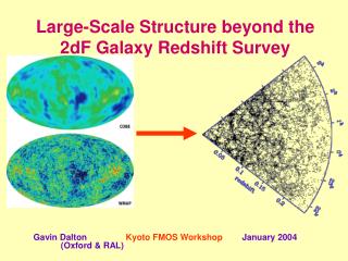
Measuring large-scale structure in the universe with the 2dF Galaxy Redshift Survey. John Peacock Garching December 2001. The distribution of the galaxies. 1930s: Hubble proves galaxies have a non-random distribution 1950s:

E N D
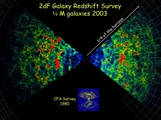
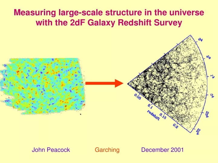
Measuring large-scale structure in the universe with the 2dF Galaxy Redshift Survey John Peacock Garching December 2001
The distribution of the galaxies 1930s: Hubble proves galaxies have a non-random distribution 1950s: Shane & Wirtanen spend 10 years counting 1000,000 galaxies by eye - filamentary patterns?
Redshift surveys Inverting v = cz = Hd gives an approximate distance. Applied to galaxies on a strip on the sky, gives a ‘slice of the universe’
Redshift surveys: v = cz = H0 d d = z x 3000 h-1 Mpc h = H0 / 100 km s-1 Mpc -1 CfA Survey ~15000 z’s Las Campanas Redshift Survey ~25000 z’s
Inflationary origin of structure? Assume early universe dominated by scalar-field V(f) at GUT energies Predicts small fluctuations in metric. Scalar fluctuations (= Newtonian potential) have nearly flat spectrum - also expect tensor modes (gravity waves)
Gravitational instability:hierarchical collapse generates ever larger structures
Nonlinear predictions of theory Bright galaxies today were assembled from fragments at high redshift
Results from the 2dF Galaxy Redshift Survey Target: 250,000 redshifts to B<19.45 (median z = 0.11) Current total: 213,000
Australia Joss Bland-Hawthorn Terry Bridges Russell Cannon Matthew Colless Warrick Couch Kathryn Deeley Roberto De Propris Karl Glazebrook Carole Jackson Ian Lewis Bruce Peterson Ian Price Keith Taylor BritainCarlton Baugh Shaun Cole Chris Collins Nick Cross Gavin Dalton Simon Driver George Efstathiou Richard Ellis Carlos Frenk Ofer Lahav Stuart Lumsden Darren Madgwick Steve Maddox The 2dFGRS Team Stephen Moody Peder Norberg John Peacock Will Percival Mark Seaborne Will Sutherland Helen Tadros 33 people at 11 institutions
2dFGRS input catalogue • Galaxies: bJ 19.45 from revised APM • Total area on sky ~ 2000 deg2 • 250,000 galaxies in total, 93% sampling rate • Mean redshift <z> ~ 0.1, almost all with z < 0.3
2dFGRS geometry ~2000 sq.deg. 250,000 galaxies Strips+random fields ~ 1x10⁸ h-3 Mpc3 Volume in strips ~ 3x10⁷ h-3 Mpc3 NGP SGP NGP 75x7.5 SGP 75x15 Random 100x2Ø ~70,000 ~140,000 ~40,000
Tiling strategy ‘2dF’ = ‘two-degree field’ = 400 spectra Efficient sky coverage, but variable completeness High completeness throughadaptive tiling:multiple coverage of high-density regions
Prime Focus The 2dF site
Now: 213000 z’s Survey Progress • 45% of nights allocated were usable • Current rate 1000 redshifts per allocated night • Survey will end in Jan 2002 after 250 nights total • Expected final size: 230,000
Sky Coverage of Survey • 62% of fields were observed up to July 2001 • Final strips will be trimmed to finish early 2002. NGP SGP
Redshift distribution • N(z) for 156000 galaxies. • Still shows significant clustering. • The median redshift of the survey is <z>=0.11 • Almost all objects have z < 0.3.
Survey mask NGP SGP Cutouts are bright stars and satellite trails.
Sampling & Uniformity • Adaptive tiling efficient, uniform sampling… when done. • At current stage of survey, sampling is highly variable. • This limits applications requiring large contiguous volumes.
Fine detail: 2-deg NGP slices (1-deg steps) 2dFGRS: bJ < 19.45 SDSS: r < 17.8
The CDM power spectrum growth: d(a) = a f(W[a]) Break scale relates to W(density in units of critical density): In practice, get shape parameter G (almost = Wh)
2dFGRS power-spectrum results Dimensionless power: d (fractional variance in density) / d ln k APM deprojection: real space 2df: redshift space result robust with respect to inclusion of random fields
2dFGRS power spectrum - detail nonlinearities, fingers of God, scale-dependent bias ... Ratio to Wh=0.25CDM model (zero baryons)
Gain x2.3 in P(k) range Power spectrum and survey window • Window sets power resolution and maximum scale probed: Pobs(k) = P(k) * |W(k)|2 • Full survey more isotropic, compact window function.
Model fitting Essential to include window convolution and full data covariance matrix
Confidence limits Wmh = 0.20 ± 0.03 Baryon fraction = 0.15 ± 0.07 ‘Prior’: h = 0.7 ± 10%
Relation to CMB results curvature baryons total density Geometrical degeneracy: need a value for h, even with no tensors
Consistency with other constraints Cluster baryon fraction Nucleo-synthesis CMB
Scalar fit to 2dFGRS + CMB Joint likelihood removes need to assume parameters: Wmh2 from CMB and Wmh from LSS gives both Wm & h: Wm = 0.27 ± 0.05
Redshift-space distortions (Kaiser 1987) zobs = ztrue + dv / c dv prop. to 0.6 dr/r = 0.6 b-1dn/n (bias) Apparent shape from below linear nonlinear
r Redshift-space clustering s p • z-space distortions due to peculiar velocities are quantified by correlation fn (,). • Two effects visible: • Small separations on sky: ‘Finger-of-God’; • Large separations on sky: flattening along line of sight
Fit quadrupole/monopole ratio of (,) as a function of r with model having 0.6/b and p (pairwise velocity dispersion) as parameters. Model fits to z-space distortions and = 0.4, p= 300,500 • Best fit for r>8h-1Mpc (allowing for correlated errors) gives: = 0.6/b = 0.43 0.07 p =385 50 km s-1 • Applies at z = 0.17, L =1.9 L* (significant corrections) • Full survey will reduce random errors in to 0.03. = 0.3,0.4,0.5; p= 400 99%
Measuring bias - 1: CMB The problem: do galaxies trace mass? dn/n = b dr/r Take mass s8 from CMB (scalar fit) and apparent (redshift-space)s8 from 2dFGRS P(k): b(1.9L*) = (1.00 ± 0.09) exp[-t + 0.5(n-1)]
2 1 2 1 3 Measuring bias - 2: Bispectrum (with Verde, Heavens, Matarrese) Two-point correlations: < d1d2 > = x : FT = P(k) power spectrum Three-point correlations: < d1d2 d3 > = z : FT = B(k1,k2,k3) bispectrum = 0 for Gaussian field. Measure of gravitational nonlinearity
Bispectrum results Assume local nonlinear bias: dg=b1dm+b2 (dm)2 Nonlinear bias can mimic some aspects of gravitational evolution (e.g. skewness) - but full bispectrum contains shape information: bias doesn’t form filaments data match unbiased predictions tCDM LCDM Results for NGP + SGP: b1= 1.04 0.11, b2= -0.05 0.08(for L=1.9L*) + b result Wm = 0.27 0.06 -entirely internal to 2dFGRS
Clustering as f(L) Clustering increases at high luminosity: b(L) / b(L*) = 0.85 + 0.15(L/L*) suggests << L* galaxies are slightly antibiased - and IRAS g’s even more so: b = 0.8
The tensor CMB degeneracy scalar plus tensors tilt to n = 1.2 raise wb to 0.03 Degeneracy: compensate for high tensors with high n and high baryon density
Constraining tensors with b Dimensionlesspower: d (fractional variance in density) / d ln k Scalar only: s8 = 0.75. Predicts b(L*) = 0.39 High tensor: s8 = 0.64. Predicts b(L*) = 0.29 (also fails to match cluster abundance)
Summary • >10 Mpc clustering in good accord with LCDM • power spectrum favours Wm h= 0.20 & 15% baryons • With h = 0.7 ± 10%, gives Wm = 0.27 ± 0.05 • No significant large-scale bias (3 arguments): • redshift-space distortions with Wmfrom P(k) • comparing CMB s8 with P(k) amplitude • direct internal bispectrum analysis • Matches no-tilt no-tensor vanilla CMB • tensor-dominated models excluded • See http://www.mso.anu.edu.au/2dFGRS/ for 100,000 redshift 2dFGRS data release