Download
1 / 39
400 likes | 634 Views
Climate-Biome Shifts in Alaska and Western Canada. Current Results and Final Steps October 2011. Participants. Scenarios Network for Alaska Planning (SNAP), University of Alaska Fairbanks EWHALE lab, Institute of Arctic Biology, University of Alaska Fairbanks US Fish and Wildlife Service

E N D
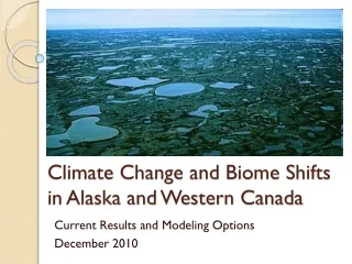
Climate-Biome Shifts in Alaska and Western Canada Current Results and Final Steps October 2011
Participants • Scenarios Network for Alaska Planning (SNAP), University of Alaska Fairbanks • EWHALE lab, Institute of Arctic Biology, University of Alaska Fairbanks • US Fish and Wildlife Service • The Nature Conservancy • Ducks Unlimited Canada • Government of the Northwest Territories • Government of Canada • Other invited experts
Overview • This project is intended to: • Develop climate and vegetation based biomes (based on cluster analysis) for AK, Yukon, NWT, and areas to the south that may represent future climatic conditions for AK,Yukon or NWT. • Model potential climate-induced biome shift. • Based on model results, identify areas that are least or most likely to change over the next 10-90 years. • Provide maps, data, and a written report summarizing, supporting, and displaying these findings. • This project builds ,and makes use of, work previously conducted by SNAP, EWHALE, USFWS, TNC, and other partners. • The completed analysis will be used by partners involved in protected areas, land use, and sustainable land use planning, e.g. connectivity.
Goals of this meeting • Review Project Goals • Summary of project background • Refresher on modeling methods and data • Update on decisions and progress thus far • Discussion and decisions from group: • Finalizing and processing results • Discuss data delivery and formats • Other issues? • Timeline for completion
The Scenarios Network for Alaska and Arctic Planning (SNAP) • SNAP is a collaborative network of the University of Alaska, state, federal, and local agencies, NGOs, and industry partners. • Its mission is to provide timely access to scenarios of future conditions in Alaska for more effective planning by decision-makers, communities, and industry.
SNAP uses data for 5 of 15 models that performed best for Alaska, Yukon, and NWT PRISM downscaled to 2 km resolution OR CRU downscaled to 10 minutes (18.4 km) Monthly temp and precip from 1900 to 2100 (historical CRU + projected) 5 models x 3 emission scenarios Available as maps, graphs, charts, raw data On line, downloadable, in Google Earth, or in printable formats No data yet: Extreme events Snowpack Coastal/Oceans SNAP Projections: based on IPCC models
Phase I: Alaska modelMapped shifts in potential biomes based on current climate envelopes for six Alaskan biomes and six Canadian Ecozones 7 http://geogratis.cgdi.gc.ca/geogratis/en/collection/detail.do?id=4361
Phase I Results:Potential Change: Current - 2100(Noting that actual species shifts lag behind climate shifts)
Improvements over Phase I • Extend scope to northwestern Canada • Use all 12 months of data, not just 2 • Eliminate pre-defined biome/ecozone categories in favor of model-defined groupings (clusters) • Eliminates false line at US/Canada border • Creates groups with greatest degree of intra-group and inter-group dissimilarity • Gets around the problem of imperfect mapping of vegetation and ecosystem types • Allows for comparison and/or validation against existing maps of vegetation and ecosystems
Other Improvements • Comparison with multiple landcover classification categories • Eliminates over-reliance on one categorization scheme • Utilizes divergent methods of classification • Recalibration of all SNAP downscaling to reconcile discontinuities between US and Canada and errors in A2 and B1 data (not used in Phase 1)* * Note that this has caused project delays, but the very extensive work involved will NOT be charged to project funders.
Cluster analysis • Cluster analysis is the assignment of a set of observations into subsets so that observations in the same cluster are similar in some sense. • Clustering is a method of “unsupervised learning” (the model teaches itself, and finds the major breaks) • Clustering is common for statistical data analysis used in many fields • The choice of which clusters to merge or split is determined by a linkage criterion (distance metrics), which is a function of the pairwise distances between observations. • Cutting the tree at a given height will give a clustering at a selected precision.
Step 1: Create a Dissimilarity Matrix • Distance measure determines how the similarity of two elements is calculated. • Some elements may be close to one another according to one distance and farther away according to another. • In our modeling efforts, all 24 variables are given equal weight, and all distances are calculated in “24-dimensional space” (similarity matrix, proximity matrix, distance matrix get converted into each other) Taxicab geometry versus Euclidean distance: The red, blue, and yellow lines have the same length in taxicab geometry for the same route. In Euclidean geometry, the green line has length 6×√2 ≈ 8.48, and is the unique shortest path.
Methods: Partitioning Around Medoids (PAM) • The dissimilarity matrix describes pairwise distinction between objects. • The algorithm PAM computes representative objects, called medoids whose average dissimilarity to all the objects in the cluster is minimal • Each object of the data set is assigned to the nearest medoid. • PAM is more robust than the well-known kmeans algorithm, because it minimizes a sum of dissimilarities instead of a sum of squared Euclidean distances, thereby reducing the influence of outliers. • PAM is a standard procedure
Resolution limitations Data are not available at the same resolution for the entire area • for Alaska, Yukon, and BC, SNAP uses 1961-1990 climatologies from PRISM, at 2 km, • for all other regions of Canada SNAP uses climatologies for the same time period from CRU, at 10 minutes lat/long (~18.4 km) • In clustering these data, both the difference in scale and the difference in gridding algorithms led to artificial incongruities across boundaries.
Solution to resolution limitations The solution to both resolution and clustering limitations was to cluster across the whole region using CRU data, which is available for the entire area, but to project future climate-biomes using PRISM, where available, to maximize resolution and sensitivity to slope, aspect, and proximity to coastlines.
How many clusters? • Choice is mathematically somewhat arbitrary, since all splits are valid • Some groupings likely to more closely match existing land cover classifications • How many clusters are defensible? • How large a biome shift is “really” a shift from the conservation perspective?
Sample cluster analysis showing 5 clusters, based on CRU 10’ climatologies. This level of detail was deemed too simplistic to meet the needs of end users.
Sample cluster analysis showing 30 clusters, based on CRU 10’ climatologies. This level of detail was deemed too complex to meet the needs of end users, as well as too fine-scale for the inherent uncertainties of the data.
Mean silhouette width for varying numbers of clusters between 3 and 50. High values in the selected range between 10 and 20 occur at 11, 17, and 18.
Eighteen-cluster map for the entire study area. This cluster number was selected in order to maximize both the distinctness of each cluster and the utility to land managers and other stakeholders.
Cluster certainty based on silhouette width. Note that certainty is lowest along boundaries.
Assessing the clusters • Box plots, rose plots, and other direct temp/precip depictions • Congruence with existing land cover classification by modal values • Congruence with land cover classification by percent
http://www.cec.org/Page.asp?PageID=924&ContentID=2819 NALCMS Land Cover, 2005 • North American Land Change Monitoring System (Canada, Mexico and US) • Based on monthly composites of 2005 MODIS imagery • 250m resolution;19 classes • Separating shrubland, grasslands, deciduous forests and evergreen forests, as well as open vs closed canopies. • Does not distinguish boreal forest, temperate forest and rain forest, and defines tundra as either “grassland” or “sparse.”
AVHRR Landcover, 1995 • USGS – NOAA data • 13 categories with clear distinctions between forest, shrubs, and grasslands. • “Dwarf shrub” and “herbaceous” categories help define tundra • Forested areas are defined primarily as deciduous or needle-leaf.
GlobCover 2009 • ESA JRC initiative • 300m MERIS sensor, ENVISAT satellite • Similar strengths and weaknesses to AVHRR
Alaska Biomes and Canadian Ecozones • Nowacki et al. 2001 and Envirnoment Canada • Differs fundamentally from other 3 classification systems -- not based on remote sensing data but rather on a combination of observed data and interpolated data. • Based on not only cover type but also functional and morphological details, e.g. ecosystem function, soil type, bedrock, wildlife.
Dominant GlobCover 2009 land cover by cluster number. All land cover categories that occur in 15% or more of a given cluster are included.
Dominant AVHRR land cover types by cluster number. All land cover categories that occur in 15% or more of a given cluster are included.
Dominant Alaska biomes and Canadian Ecozones by cluster number. Alaska biomes are adapted from Nowacki et al. 2001; Canadian ecozones are definedby Natural Resources Canada. All categories that occur in 15% or more of a given cluster are included.
Climate-biome characteristics • Mixed boreal forest, interior climate • Boreal forest with coastal influence and intermixed grass and tundra • Cold northern boreal/subarctic forest • More densely forested closed-canopy boreal • Dry, sparsely vegetated northern boreal • Interior boreal, densely forested • Warmer boreal zone with mixed evergreen and deciduous • Southern boreal, mixed forest • Coastal rainforest, wet, more temperate • Prairie and grasslands • The coldest cliome. Northern Arctic sparsely vegetated tundra with up to 25% bare ground and ice, with an extremely short growing season. • Cold northern arctic tundra, but primarily vegetated • More densely vegetated arctic tundra with up to 40% shrubs but no tree cover • Arctic tundra with denser vegetation, a longer growing season, and more shrub cover including some small trees • Dry sparsely vegetated southern arctic tundra • Northern boreal/southern arctic shrubland, with an open canopy and short growing season • Northern boreal coniferous woodland, open canopy • Dry boreal wooded grasslands — mixed coniferous forests and grasses
Data selected from SNAP models Available climate data from SNAP includes output for each of the five best-performing GCMs as well as a composite (mean) of all five models for all months of all years to 2100, for each of three emission scenarios as defined by the IPCC: A1B, A2, B1 • Selected three future time periods (2030-2039; 2060-2069 and 2090-2099). Decadal averages deemed more useful than single years for capturing trends. • Chose to provide outputs from all five models plus composite in A1B, and all three emission scenarios with composite.
Defining refugia and areas of greatest change • Decadal results from RandomForest will be analyzed to determine which grid cells are projected to remain within the same biome climate envelope over the time periods. • Thresholds for what constitutes greatest change • Sites that shift climatically to match non-adjacent biomes can be interpreted as a proxy for magnitude of change • Areas that shift to a climate-biome with different dominant land cover types according to AVHRR, GlobCover, etc.
Interpreting confidence in refugia/ areas of change • Only consider areas selected as refugia in the majority (or all?) of the climate models • RandomForest assigns a ranking value to each of pixel that can be used to identify the model confidence • Treat boundary zones (low silhouette values) between cliomes as belonging to either cliome
Data and Product Delivery • Formal report • Report submitted to the FWS Journal of Fish & Wildlife Management or to a peer reviewed journal • Executive summary • Additional short/simplified/regional versions? • PPT presentations – for what audiences? • Posters, talks, and additional publications?
Timeline for completion • Remaining salary provided by grants will not be withdrawn until project completion • Remaining modeling/mapping steps • Finalizing projection results • Defining refugia/areas of change • Hoping to meet current Dec 31 goal • Product creation • Simultaneous with above • Likely to require group feedback, final edits, copy editing and printing in early 2012