Download

1 / 26
260 likes | 324 Views
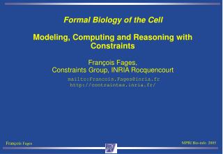
Formal Biology of the Cell Modeling, Computing and Reasoning with Constraints François Fages, Constraint Programming Group, INRIA Rocquencourt mailto:Francois.Fages@inria.fr http://contraintes.inria.fr/. Overview of the Lectures. Introduction. Formal molecules and reactions in BIOCHAM.

E N D
Formal Biology of the CellModeling, Computing and Reasoning with ConstraintsFrançois Fages, Constraint Programming Group, INRIA Rocquencourtmailto:Francois.Fages@inria.frhttp://contraintes.inria.fr/
Overview of the Lectures • Introduction. Formal molecules and reactions in BIOCHAM. • Formal biological properties in temporal logic. Symbolic model-checking. • Continuous dynamics. Kinetics models. • Computational models of the cell cycle control [L. Calzone]. • Mixed models of the cell cycle and the circadian cycle [L. Calzone]. • Machine learning reaction rules from temporal properties. • Constraint-based model checking. Learning kinetic parameter values. • Constraint Logic Programming approach to protein structure prediction.
A Logical Paradigm for Systems Biology • Biological property = Temporal Logic Formula • Biological validation = Model-checking • Initial state : experimental conditions, wild-life/mutated organisms,… • reachable(P)==EF(P) • checkpoint(s2,s)== E(s2U s) • stable(s)== AG(s) • steady(s)==EG(s) • oscil(P)== EG((P EF P) ^ (P EF P)) • Reach threshold concentration : F([M]>0.2) On derivative : F(d([M])>0.2) • Reach and stays above threshold : FG([M]>0.2) • oscil(P,n)==F(d([M])/dt>0 & F(d([M])/dt<0 & … )) n times
Kripke Semantics of CTL • A Kripke structure K is a triple (S,R) where S is a set of states, and RSxS is a total relation. • s |= f if propositional formula f is true in s, • s |= E f if there is a path from s such that |= f, • s |= A f if for every path from s, |= f, • |= f if s |= f where s is the starting state of , • |= X f if 1 |= f, • |= F f if there exists k ≥ 0 such that k |= f, • |= G f if for every k ≥ 0, k |= f, • |= f1 U f2 iff there exists k>0 such that k |= f for all j < k j |= f. • Following [Emerson 90] we identify a formula f to the set of states which satisfy it f ~ {sS : s |= f}.
CTL Equivalence of Boolean Models • For a class C of CTL formulae, • given two Kripke structures K=(S,R), K’=(S,R’) and an initial state s • K ~C K’ iff {fC : K,s|=f} = {fC : K’,s|=f} • Which model transformations preserve a class of CTL properties? • Model refinement or simplification preserving a CTL specification • Which model transformations can make a CTL property true? • Learning of rules to add or to delete to satisfy a CTL specification • Which CTL properties are satisfied by a Biocham model? genCTL(pattern)
CTL Equivalence for a Simple Enzymatic Reaction • Two Biocham models: M1={A+B<=>D, D=>A+C} or M2={B =[A]=> C} • D having no other occurrence in M1. • Let f and ψ be two propositional formulae. • Proposition If M2 |= EF(f) then M1 |= EF(f).Moreover, if A and B do not appear negatively (i.e. under an odd number of negations) in f and D does not appear at all in f, then M1 |= EF(f) implies M2 |= EF(f). • Proposition If A and B do not appear negatively in ψ and D does not appear in ψ,then M2 |= ¬E(¬fU ψ) implies M1 |= ¬E(¬fU ψ). If A and B do not appear negatively in f and D does not appear in f,then M1 |= ¬E(¬fU ψ) implies M2 |= ¬E(¬fU ψ).
Positive and Negative CTL Formulae • Let K = (S,R,L) and K’ = (S,R’,L) be two Kripke structures such that RR’ • . • Def. An ECTL (positive) formula is a CTL formula with no occurrence of A (nor negative occurrence of E). • Def. An ACTL (negative) formula is a CTL formula with no occurrence of E (nor negative occurrence of A). • Proposition For any ECTL formula f, if K’ |≠ f then K |≠ f. • Since RR’ all paths in K are also paths in K’, hence for a positive formula f, if K |= f then K’ |= f, which shows the proposition. • Proposition For any ACTL formula f, if K |≠ f then K’ |≠ f. • By duality ¬f is a positive formula, hence if K |= ¬f then K’ |= ¬f.
Example of Qu’s Model of Cell Cycle • _=>Cyclin. • Cyclin=>_. • Cyclin+Cdc2~{p1}=>Cdc2~{p1}-Cyclin~{p1}. • Cdc2~{p1}-Cyclin~{p1}=>Cdc2-Cyclin~{p1}. • Cdc2~{p1}-Cyclin~{p1}=[Cdc2-Cyclin~{p1}]=>Cdc2-Cyclin~{p1}. • Cdc2-Cyclin~{p1}=>Cdc2~{p1}-Cyclin~{p1}. • Cdc2-Cyclin~{p1}=>Cdc2+Cyclin~{p1}. • Cyclin~{p1}=>_. • Cdc2=>Cdc2~{p1}. • Cdc2~{p1}=>Cdc2. • present(Cdc2,1). make_absent_not_present.
Aut. Generation of a CTL Specification in Qu’s Model • Enumerate all CTL formulae (of some pattern) that are true in a model. • ? genCTL(elementary_properties). • Ai(oscil(C25)), • Ei(reachable(C25~{p1})), Ei(reachable(!(C25~{p1}))), Ai(oscil(C25~{p1})), • Ei(reachable(Wee1)), Ei(reachable(!(Wee1))), Ai(oscil(Wee1)), • Ei(reachable(Wee1~{p1})),Ei(reachable(!(Wee1~{p1}))), Ai(oscil(Wee1~{p1})), • Ai(AG(!(Wee1~{p1})->checkpoint(Wee1,Wee1~{p1}))), • Ei(reachable(CKI)), Ei(reachable(!(CKI))), Ai(oscil(CKI)), • Ei(reachable(CKI-CycB-CDK~{p1})),Ei(reachable(!(CKI-CycB-CDK~{p1}))), • Ai(oscil(CKI-CycB-CDK~{p1})), • Ei(reachable((CKI-CycB-CDK~{p1})~{p2})), Ei(reachable(!((CKI-CycB-CDK~{p1})~{p2}))), • Ai(oscil((CKI-CycB-CDK~{p1})~{p2})), Ai(AG(!((CKI-CycB-CDK~{p1})~{p2}) • ->checkpoint(CKI-CycB-CDK~{p1},CKI-CycB-CDK~{p1})~{p2}))}).
Generation of Rule Additions for a CTL Specification • Enumerate all rules (of some pattern) that satisfy a CTL specification • ? delete_rule(Cyclin+Cdc2~{p1}=>Cdc2~{p1}-Cyclin~{p1}). • ? learn_one_addition(elementary_interaction_rules). • (1) Cyclin+Cdc2~{p1}=[Cdc2]=>Cdc2~{p1}-Cyclin~{p1} • (2) Cyclin+Cdc2~{p1}=[Cyclin]=>Cdc2~{p1}-Cyclin~{p1} • (3) Cyclin+Cdc2~{p1}=>Cdc2~{p1}-Cyclin~{p1} • (4) Cyclin+Cdc2~{p1}=[Cdc2~{p1}]=>Cdc2~{p1}-Cyclin~{p1} • Similarly enumerate all rule deletions that satisfy or preserve a CTL spec. • ? learn_one_deletion(reaction_pattern, spec_CTL) • ? reduce_model(spec_CTL)
Learning Model Revision from Temporal Properties • Theory T: BIOCHAM model • molecule declarations • interaction rules: complexation, phosphorylation, … • Examples φ: CTL specification of biological properties • Reachability • Checkpoints • Stable states • Oscillations • Bias R: Rule pattern • Kind of rules to add or delete • Find a revision T’ of T such that T’ |= φ
Theory Revision Algorithm • General idea of constraint programming: replace a generate-and-test algorithm by a constrain-and-generate algorithm. • Anticipate whether one has to add or remove a rule? • Positive ECTL formula: if false, remains false after removing a rule • EF(φ) where φ is a boolean formula (pure state description) • Negative ACTL formula: if false, remains false after adding a rule • AG(φ) where φ is a boolean formula, • Checkpoint(a,b): ¬E(¬aUb) • Remove a rule on the path given by the model checker (why command) • Unclassified CTL formulae • Loop(a)= AG((a EFa)^(a EFa))
Theory Revision Algorithm Rules • Initial state: <(0, 0, 0), (E,U,A), R> • E transition: <(E,U,A), (E{e},U,A), R> <(E{e},U,A), (E,U,A),R> if R |= e • E’ transition: <(E,U,A), (E {e},U,A), R> <(E{e},U,A), (E,U,A),R {r}> • if R |≠ e and f {e} EUA, K {r} |= f
Theory Revision Algorithm Rules • Initial state: <(0, 0, 0), (E,U,A), R> • E transition: <(E,U,A), (E{e},U,A), R> <(E{e},U,A), (E,U,A),R> if R |= e • E’ transition: <(E,U,A), (E {e},U,A), R> <(E{e},U,A), (E,U,A),R {r}> • if R |≠ e and f {e} EUA, K {r} |= f • U transition: <(E,U,A), (0,U {u},A), R > <(E,U {u},A), (0,U,A),R> if R |= u • U’ transition: <(E,U,A), (0,U {u},A), R > <(E,U{u},A), (0,U,A),R {r}> • if R|≠u and f {u} EUA, R {r} |= f • U” transition: <(E,U,A), (0,U {u},A), R Re > <(E,U{u},A),(0,U,A), R> • if K,si|≠u and f {u} EUA, R |= f
Theory Revision Algorithm Rules • Initial state: <(0, 0, 0), (E,U,A), R> • E transition: <(E,U,A), (E{e},U,A), R> <(E{e},U,A), (E,U,A),R> if R |= e • E’ transition: <(E,U,A), (E {e},U,A), R> <(E{e},U,A), (E,U,A),R {r}> • if R |≠ e and f {e} EUA, K {r} |= f • U transition: <(E,U,A), (0,U {u},A), R > <(E,U {u},A), (0,U,A),R> if R |= u • U’ transition: <(E,U,A), (0,U {u},A), R > <(E,U{u},A), (0,U,A),R {r}> • if R|≠u and f {u} EUA, R {r} |= f • U” transition: <(E,U,A), (0,U {u},A), R Re > <(E,U{u},A),(0,U,A), R> • if K,si|≠u and f {u} EUA, R |= f • A transition: <(E,U,A), (0, 0,A {a}), R > <(E,U,A{a}), (Ep,Up,A),R> if R |= a • A’ transition: <(EEp,UUp,A),(0,0,A{a}), RRe><(E,U,A{a}),(Ep,Up,A),R> if R|≠ a, f {u} [ E U A, R |= f and Ep Up is the set of formulae no longer satisfied after the deletion of the rules in Re.
Termination and Correctness • Proposition The model revision algorithm terminates. If the terminal configuration • is of the form < (E,U,A), (0,0,0), R > then the model R satisfies the • initial CTL specification. • Proof The termination of the algorithm is proved by considering the lexicographic • ordering over the couple < a, n > where a is the number of unsatisfied • ACTL formulae, and n is the number of unsatisfied ECTL and UCTL formulae. • Each transition strictly decreases either a, or lets a unchanged and strictly • decreases n. • The correction of the algorithm comes from the fact that each transition • maintains only true formulae in the satisfied set, and preserves the complete • CTL specification in the union of the satisfied set and the untreated set.
Incompleteness • Two reasons: • The satisfaction of ECTL and UCTL formula is searched by adding only one rule to the model (transition E’ and U’) • The Kripke structure associated to a Biocham set of rules adds loops on terminal states. Hence adding or removing a rule may have an opposite deletion or addition of the loops. • Just a heuristic algorithm…
Example in Qu’s Model of Cell Cycle • biocham:add_spec(Ai(AG((CycB-CDK~{p1})) • ->checkpoint(C25~{p1,p2},CycB-CDK~{p1})))). • biocham: revise_model. • Success • Time: 441.00 s • 40 properties treated • Modifications found: • Deletion(s): • k5*[CycB-CDK~{p1,p2}] for CycB-CDK~{p1,p2}=>CycB-CDK~{p1}. • k15*[CKI-CycB-CDK~{p1}] for CKI-CycB-CDK~{p1}=>CKI+CycB-CDK~{p1}. • Addition(s):
Example of Model Refinement • ? Add_spec({ Ei(reachable(CycE)), Ei(reachable(CycE-CDKp)), • Ei(reachable(CycE-CDKp~{p1})), Ei(reachable(CKI-CycE-CDKp)), Ei(reachable(!(CKI-CycE-CDKp))), Ai(oscil(CycE-CDKp)), Ai(oscil(CycE-CDK~{p1})), Ai(loop(CycE-CDKp,(CycE-CDKp)~{p1}))}). • ? Revise_model. • Deletion(s): • Addition(s): • CKI+CycE-CDKp=>CKI-CycE-CDKp. • CDKp+CycE=>CycE-CDKp. • CycE-CDKp=>(CycE-CDK)~{p1}. • (CycE-CDKp)~{p1}=>CycE-CDKp. • CKI+CycE-CDKp=>CKI-CycE-CDKp.
Rule Inference in Cell Cycle Control • [Tyson et al. 91] model over 6 variables, • initial state present(cdc2). • _ => cyclin. • cdc2˜{p} + cyclin => cdc2˜{p}-cyclin˜{p}. • cdc2˜{p}-cyclin˜{p} =>cdc2-cyclin˜{p}. ERASED • cdc2-cyclin˜{p} => cdc2 + cyclin˜{p}. • cyclin˜{p} => _. • cdc2 <=> cdc2˜{p}.
Rule Inference in Cell Cycle Control (cont.) • CTL specification of biological properties: • Activation of the kinase-cyclin (MPF) complex • reachable(cdc2-cyclin˜{p}). • Oscillation of the cycle’s phase: • loop(cyclin & cyclin˜{p} & !(cdc2-cyclin˜{p})).
Rule Inference in Cell Cycle Control (cont.) • ? learn([$Q=>$P where $P in complexes and $Q in complexes]). • _=>cdc2-cyclin˜{p} • cyclin=>cdc2-cyclin˜{p} • cdc2˜{p}-cyclin˜{p}=>cdc2-cyclin˜{p} • ? learn([$qp=>$q where $q in complexes and $qp modif $q]). • cdc2˜{p}-cyclin˜{p}=>cdc2-cyclin˜{p} • Adding temporal specification checkpoint(cdc2˜{p},cdc2-cyclin˜{p}). • ? learn([$Q=>$P where $P in complexes and $Q in complexes]). • cdc2˜{p}-cyclin˜{p}=>cdc2-cyclin˜{p}
Model Refinement by Theory Revision • Hypothetical model of three proteins MA, MB, MC • reachable(MA), reachable(MB), reachable(MC). • reachable(¬MA), reachable(¬MB), reachable(¬MC). • Oscillations are observed experimentally. • loop(MA), loop(MB), loop(MC). • Interactions between protein are unknown. • Simplest boolean model: • _<=>MA. • _<=>MB. • _<=>MC.
Model Refinement by Theory Revision (cont.) • MC is needed for the disappearance of MB: checkpoint(MC,!MB). • ? checkpoint(MC,!MB). • false • ? Why. • … MB=>_ … • ? delete_rules(MB=>_). • ? learn(elementary_interaction_pattern). • MB+MC=>MB˜{p}+MC. • MB+MC=>MC. • MB+MC=>MB-MC. • ? Add_rule(MB+MC=>MB˜{p}+MC).
Model Refinement by Theory Revision (cont.) • MA is needed for the disappearance of MC: checkpoint(MA,!MC). • ? checkpoint(MA,!MC). • False • ? Why • … MC => _ … • ? delete_rule(MC => _ ). • ? Learn(elementary_interaction_pattern(MC)). • MC+MA=>MA-MC • MC+MA=>MC~{p}+MA • MC+MA=>MA • ? Add_rule(MC+MA=>MC~{p}+MA ).
Model Refinement by Theory Revision (cont.) • MB is needed for the disappearance of MA: checkpoint(MB,!MA). • ? checkpoint(MB,!MA). • False • ? Why • … MA => _ … • ? delete_rule(MA => _ ). • ? Learn(elementary_interaction_pattern(MA)). • MC+MA=>MA-MC MC+MA=>MC~{p}+MA MC+MA=>MA • ? Add_rule(MC+MA=>MC~{p}+MA ). • _=>MA. • MA=[MB]=>_. • _=>MB. • MB=[MC]=>MB˜{p}. • _=>MC. • MC=[MA]=>MC˜{p}.