Download
1 / 47
470 likes | 662 Views
Plotting & Interpreting Multiple Regression Models. Why plot MR models? Interpretive review & extensions Plotting single-predictor models centered quant, binary or k-category predictors Plotting two-predictor models centered quant & binary, k-category or centered quant

E N D
Plotting & Interpreting Multiple Regression Models • Why plot MR models? • Interpretive review & extensions • Plotting single-predictor models • centered quant, binary or k-category predictors • Plotting two-predictor models • centered quant & binary, k-category or centered quant • Plotting multiple-predictor models
So far we have emphasized the clear interpretation of regression weights for each type of predictor. • Many of the “more complicated” regression models, such as ANCOVA or those with non-linear or interaction terms are plotted, because, as you know, “a picture is worth a lot of words”. • Each term in a multiple regression model has an explicit representation in a regression plot as well as an explicit interpretation – usually with multiple parallel phrasing versions. • So, we’ll start simple with simple models and learn the correspondence between: • interpretation of each regression model term • the graphical representation of that term
Coding & Transforming predictors for MR models • Categorical predictors will be converted to dummy codes • comparison/control group coded 0 • @ other group a “target group” of one dummy code, coded 1 • Quantitative predictors will be centered, usually to the mean • centered = score – mean (like for quadratic terms) • so, mean = 0 Why? Mathematically – 0s (as control group & mean) simplify the math & minimize collinearity complications Interpretively – the “controlling for” included in multiple regression weight interpretations is really “controlling for all other variables in the model at the value 0” – “0” as the comparison group & mean will make b interpretations simpler and more meaningful
Very important things to remember… • 1) We plot and interpret the model of the data -- not the data • if the model fits the data poorly, then we’re carefully describing and interpreting nonsense • 2) The interpretation of regression weights in a main effects model is different than in a model including interactions • regression weights reflect “main effects” in a main effects model (without interactions) • regression weights reflect “simple effects” in a model including interactions
Models with a single quantitative predictor y’ = bX + a • a regression constant • expected value of y if x = 0 • height of predictor-criterion regression line • b regression weight • expected direction and extent of change in y for a 1-unit increase in x • slope of line
Graphing & Interpreting Models with a single quantitative predictor y’ = bX + a a = height of line b = slope of line 0 10 20 30 40 50 60 Y a + b 0 10 20 30 40 X
Models with a single centered quantitative predictor Xcen = X – Xmean y’ = bXcen + a • a regression constant • expected value of y when x = 0 (x = mean) • height of predictor-criterion regression line • b regression weight • expected direction and extent of change in y for a 1-unit increase in x • slope of predictor-criterion regression line X will be Xcen in all of the following models
Models with a single centered quantitative predictor y’ = bXcen + a Xcen = X – Xmean • So, how do we plot this formula? • Simple pick 2 values of xcen, substitute them into the formula to get y’ values and plot the line defined by those two x-y points • What x values? • doesn’t matter -- so keep it simple… • 0 & 1, 0 & 10, 0 & 100, depending on the x-scale • +/- 2 std isn’t as simple, but tells you what x & y ranges are needed on the plot • Couple of things to remember… • “0” is the center of the x-axis – X has been centered !!! • the x-axis should extend about +/- 2 Std (include 96% of pop)
Models with a single centered quantitative predictor y’ = 1.5X + 30 If X has mean = 42 & std = 7.5 For +2std1.6*15 + 30 y’ = 54 For -2std1.6*-15 + 30 y’ = 6 For xcen = 01.6*0 + 30 y’ = 30 For xcen = 101.6*10 + 30 y’ = 46 Any set of x values will lead to the same plotted line! 0 10 20 30 40 50 60 70 We can even substitute the original x scale back into the graph !! -20 -10 0 10 20 Xcen 20 30 40 50 60 X
Graphing & Interpreting Models with a single centered quantitative predictor Xcen = X – Xmean y’ = bXcen + a a = ht of line b = slp of line 0 10 20 30 40 50 60 +b a (x = mean) -20 -10 0 10 20 Xcen
Graphing & Interpreting Models with a single centered quantitative predictor Xcen = X – Xmean y’ = bXcen + a a = ht of line b = slp of line b = 0 0 10 20 30 40 50 60 a (x = mean) -20 -10 0 10 20 Xcen
Graphing & Interpreting Models with a single centered quantitative predictor Xcen = X – Xmean y’ = -bXcen + a a = ht of line b = slp of line 0 10 20 30 40 50 60 -b a (x = mean) -20 -10 0 10 20 Xcen
Models with a single binary predictor coded 1-2 y’ = bX + a • a regression constant • expected value of y if x = 0 (no one has this value – all coded 1 or 2) • height of line • b regression weight • expected direction and extent of change in y for a 1-unit increase in x • direction and extent of y mean difference between groups coded 1 & 2 • slope of line
Plotting & Interpreting models with a single binary predictor coded 1-2 y’ = bZ + a Z = Tx1 vs. Cx Cx = 1 Tx = 2 +b 0 10 20 30 40 50 60 Control Tx1
Plotting & Interpreting models with a single binary predictor coded 1-2 y’ = bZ + a Z = Tx1 vs. Cx Cx = 1 Tx = 2 b = 0 0 10 20 30 40 50 60 Control Tx1
Plotting & Interpreting models with a single binary predictor coded 1-2 y’ = -bZ + a Z = Tx1 vs. Cx Cx = 1 Tx = 2 -b 0 10 20 30 40 50 60 Control Tx1
Models with a single dummy coded binarypredictor y’ = bZ + a • a regression constant • expected value of y if z = 0 (the control group) • mean of the control group • height of control group • b regression weight • expected direction and extent of change in y for a 1-unit increase in x • direction and extent of y mean difference between groups coded 0 & 1 • group height difference The way we’re going to graph this model looks strange, but will provide simplicity & clarity for more complex models.
Plotting & Interpreting Models with a single dummy coded binarypredictor y’ = bZ + a Z = Tx1 vs. Cx Cx = 0 Tx = 1 a = ht Cx b = htdif Cx & Tx Tx 0 10 20 30 40 50 60 + b Cx a
Plotting & Interpreting Models with a single dummy coded binarypredictor y’ = bZ + a Z = Tx1 vs. Cx Cx = 0 Tx = 1 a = ht Cx b = htdif Cx & Tx 0 10 20 30 40 50 60 Tx b = 0 Cx a
Plotting & Interpreting Models with a single dummy coded binarypredictor y’ = -bZ + a Z = Tx1 vs. Cx Cx = 0 Tx = 1 a = ht Cx b = htdif Cx & Tx a Cx 0 10 20 30 40 50 60 - b Tx
Models with a single k-category predictor coded 1-3 Can’t put the 1-3 coded variable into a regression – not a quant/interval variable y’ = bX + a 0 10 20 30 40 50 60 Control Tx1 Tx2
Models with a dummy coded k-categorypredictor – 2 dummy codes Group Z1 Z2 1 1 0 2 0 1 3*0 0 y’ = b1Z1 + b2Z2 + a • a regression constant • expected value of y if Z1 & Z2 = 0 (the control group) • mean of the control group • height of control group • b1 regression weight related to group 1 vs. target group • expected direction and extent of change in y for a 1-unit increase in x • direction and extent of y mean difference between comparison group and target group coded 1 on this variable • group height difference between comparison & target groups (3 & 1) • b2 regression weight related to group 2 vs. target group • expected direction and extent of change in y for a 1-unit increase in x • direction and extent of y mean difference between comparison group and target group coded 1 on this variable • group height difference between comparison & target groups (3 & 2) The way we’re going to graph this model looks strange, but will provide simplicity & clarity for more complex models.
Plotting & Interpreting Models with a dummy coded k-category predictor – 2 dummy codes y’ = b1Z1 + b2Z2 + a Z1 = Tx1 vs. Cx(0) Z2 = Tx2 vs. Cx(0) a = ht Cx Tx2 b1 = htdif Cx & Tx1 b2 = htdif Cx & Tx2 + b2 Tx1 0 10 20 30 40 50 60 + b1 Cx a
Plotting & Interpreting Models with a dummy coded k-category predictor – 2 dummy codes y’ = b1Z1 + b2Z2 + a Z1 = Tx1 vs. Cx(0) Z2 = Tx2 vs. Cx(0) a = ht Cx b1 = htdif Cx & Tx1 b2 = htdif Cx & Tx2 0 10 20 30 40 50 60 Tx2 Tx1 b2=0 Cx b1=0 The dots should overlap – but that makes it hard to see… a
Plotting & Interpreting Models with a dummy coded k-category predictor – 2 dummy codes y’ = -b1Z1 + b2Z2 + a Z1 = Tx1 vs. Cx(0) Z2 = Tx2 vs. Cx(0) a a = ht Cx Cx b1 = htdif Cx & Tx1 b2 = 0 Tx2 b2 = htdif Cx & Tx2 0 10 20 30 40 50 60 - b1 Tx1 The top 2 dots should overlap – but that makes it hard to see…
Now we get to the fun part – plotting multiple regression equations involving multiple variables. • Three kinds (for now, more later) … • centered quant variable & dummy-coded binary variable • centered quant variable & dummy-coded k-category variable • 2 centered quant variables What we’re trying to do is to plot these models so that we can see how both of the predictors are related to the criterion. Like when we’re plotting data from a factorial design, we have to represent 3 variables -- the criterion & the 2 predictors X & Z -- in a 2-dimensional plot. We’ll use the same solution.. We’ll plot the relationship between one predictor and the criterion for different values of the other predictor
Models with a centered quantitative predictor & a dummy coded binary predictor This is called a main effects model there are no interaction terms. y’ = b1X + b2Z + a • a regression constant • expected value of y if X=0 (mean) and Z=0 (comparison group) • mean of the control group • height of control group quant-criterion regression line • b1 regression weight for centered quant predictor – main effect of X • expected direction and extent of change in y for a 1-unit increase in x , after controlling for the other variable(s) in the model • expected direction and extent of change in y for a 1-unit increase in x , for the comparison group (coded 0) • slope of quant-criterion regression line for the group coded 0 (comp) • b2 regression weight for dummy coded binary predictor – main effect of Z • expected direction and extent of change in y for a 1-unit increase in x, after controlling for the other variable(s) in the model • direction and extent of y mean difference between groups coded 0 & 1, after controlling for the other variable(s) in the model • group mean/reg line height difference (when X = 0, the centered mean)
To plot the model we need to get separate regression formulas for each Z group. We start with the multiple regression model… Model y’ = b1X + b2Z + a For the Comparison Group coded Z = 0 Substitute the 0 in for Z Simplify the formula y’ = b1X + b2*0 + a y’ = b1X + a slope height For the Target Group coded Z = 1 Substitute the 1 in for Z Simplify the formula y’ = b1X + b2*1 + a y’ = b1X + ( b2 + a) slope height
Plotting & Interpreting Models with a centered quantitative predictor & a dummy coded binary predictor y’ = b1X + b2 Z + a This is called a main effects model no interaction the regression lines are parallel. Xcen = X – Xmean Z = Tx1 vs. Cx(0) a= ht of Cx line mean of Cx b1 = slp of Cx line Cx slp = Tx slp No interaction 0 10 20 30 40 50 60 b1 Tx b2 b2= htdif Cx & Tx Cx & Tx mean dif a Cx -20 -10 0 10 20 Xcen
Plotting & Interpreting Models with a centered quantitative predictor & a dummy coded binary predictor This is called a main effects model no interaction the regression lines are parallel. y’ = -b1X + -b2 Z + a Xcen = X – Xmean Z = Tx1 vs. Cx(0) a= ht of Cx line mean of Cx b1 = slp of Cx line Cx slp = Tx slp No interaction 0 10 20 30 40 50 60 -b1 b2 = 0 Tx b2= htdif Cx & Tx Cx & Tx mean dif a Cx -20 -10 0 10 20 Xcen
Plotting & Interpreting Models with a centered quantitative predictor & a dummy coded binary predictor This is called a main effects model no interaction the regression lines are parallel. y’ = b1X + b2 Z + a Xcen = X – Xmean Z = Tx1 vs. Cx(0) a= ht of Cx line mean of Cx b1 = slp of Cx line Tx b1 = 0 Cx slp = Tx slp No interaction 0 10 20 30 40 50 60 b2 Cx b2= htdif Cx & Tx Cx & Tx mean dif a a -20 -10 0 10 20 Xcen
This is called a main effects model there are no interaction terms. Models with a centered quantitative predictor & a dummy coded k-category predictor y’ = b1X + b2Z1+ b3Z2+ a Group Z1 Z2 1 1 0 2 0 1 3*0 0 • a regression constant • expected value of y if Z1 & Z2 = 0 (the control group) • mean of the control group • height of control group quant-criterion regression line • b1 regression weight for centered quant predictor – main effect of X • expected direction and extent of change in y for a 1-unit increase in x • slope of quant-criterion regression line (for both groups) • b2 regression weight for dummy coded comparison of G1 vs G3 – main effect • expected direction and extent of change in y for a 1-unit increase in x • direction and extent of y mean difference between groups 1 & 3 • group height difference between comparison & target groups (3 & 1)(X = 0) • b3 regression weight for dummy coded comparison of G2 vs. G3 – main effect • expected direction and extent of change in y for a 1-unit increase in x • direction and extent of y mean difference between groups coded 0 & 1 • group height difference between comparison & target groups (3 & 2)(X = 0)
To plot the model we need to get separate regression formulas for each Z group. We start with the multiple regression model… Model y’ = b1X + b2Z1 + b3Z2 + a Group Z1 Z2 1 1 0 2 0 1 3*0 0 For the Comparison Group coded Z1= 0 & Z2 = 0 Substitute the Z code values y’ = b1X + b2*0 + b3*0 + a Simplify the formula y’ = b1X + a height slope For the Target Group coded Z1= 1 & Z2 = 0 Substitute the Z code values y’ = b1X + b2*1 + b3*0 + a Simplify the formula y’ = b1X + (b2 + a) height slope For the Target Group coded Z1= 0 & Z2 = 1 Substitute the Z code values y’ = b1X + b2*0 + b3*1 + a Simplify the formula y’ = b1X + (b3 + a) height slope
Plotting & Interpreting Models with a centered quantitative predictor & a dummy coded k-category predictor This is called a main effects model no interaction the regression lines are parallel. y’ = b1X + -b2Z1+ b3Z2+ a Xcen = X – Xmean Z1 = Tx1 vs. Cx(0) Z2 = Tx2 vs. Cx (0) a= ht of Cx line mean of Cx b1 = slp of Cx line b3 Tx2 Cx slp = Tx1 slp = Tx2 slp No interaction 0 10 20 30 40 50 60 Cx b1 -b2 b2= htdif Cx & Tx1 Cx & Tx1 mean dif Tx1 a b3= htdif Cx & Tx2 Cx & Tx2 mean dif -20 -10 0 10 20 Xcen
Plotting & Interpreting Models with a centered quantitative predictor & a dummy coded k-category predictor This is called a main effects model no interaction the regression lines are parallel. y’ = b1X + b2Z1+ b3Z2+ a Z1 = Tx1 vs. Cx(0) Z2 = Tx2 vs. Cx (0) Xcen = X – Xmean a= ht of Cx line mean of Cx Tx2 b1 = slp of Cx line b1 = 0 Cx slp = Tx1 slp = Tx2 slp No interaction 0 10 20 30 40 50 60 b3 Tx1 b2= htdif Cx & Tx1 Cx & Tx1 mean dif Cx b2 = 0 a b3= htdif Cx & Tx2 Cx & Tx2 mean dif -20 -10 0 10 20 Xcen
Plotting & Interpreting Models with a centered quantitative predictor & a dummy coded k-category predictor This is called a main effects model no interaction the regression lines are parallel. y’ = -b1X + b2Z1+ b3Z2+ a Z1 = Tx1 vs. Cx(0) Z2 = Tx2 vs. Cx (0) Xcen = X – Xmean a= ht of Cx line mean of Cx Tx1 Cx b1 = slp of Cx line b3 Tx2 Cx slp = Tx1 slp = Tx2 slp No interaction b2 = 0 0 10 20 30 40 50 60 b2= htdif Cx & Tx1 Cx & Tx1 mean dif a a b3= htdif Cx & Tx2 Cx & Tx2 mean dif -b1 -20 -10 0 10 20 Xcen
weights for main effects models w/ a centered quantitative predictor & a dummy coded binary predictor ora dummy coded k-category predictor • Constant “a” • the expected value of y when the value of all predictors = 0 • height of the Y-X regression line for the comparison group • b for a centered quantitative variable – main effect • the direction and extent of the expected change in the value of y for a 1-unit increase in that predictor, holding the value of all other predictors constant at 0 • slope of the Y-X regression line for the comparison group • b for a dummy coded binary variable -- main effect • the direction and extent of expected mean difference of the Target group from the Comparison group, holding the value of all other predictors constant at 0 • difference in height of the Y-X regression lines for the comparison & target groups • comparison & target groups Y-X regression lines have same slope – no interaction • b for a dummy coded k-group variable – main effect • the direction and extent of the expected mean difference of the Target group for that dummy code from the Comparison group, holding the value of all other predictors constant at 0 • difference in height of the Y-X regression lines for the comparison & target groups • comparison & target groups Y-X regression lines have same slope – no interaction
Models with 2 centered quantitative predictors This is called a main effects model there are no interaction terms. y’ = b1X + b2Z + a • Same idea … • we want to plot these models so that we can see how both of the predictors are related to the criterion • Different approach … • when the second predictor was binary or had k-categories, we plotted the Y-X regression line for each Z group • now, however, we don’t have any groups – both the X & Z variables are centered quantitative variables • what we’ll do is to plot the Y-X regression line for different values of Z • the most common approach is to plot the Y-X regression line for… • the mean of Z • +1 std above the mean of Z • -1 std below the mean of Z We’ll plot 3 lines
Models with 2 centered quantitative predictors This is called a main effects model there are no interaction terms. y’ = b1X1 + b2X2 + a • a regression constant • expected value of y if X=0 (mean) Z=0 (mean) • mean criterion score of those having Z=0 (mean) • height of quant-criterion regression line for those with Z=0 (mean) • b1 regression weight for X1 centered quant predictor • expected direction and extent of change in y for a 1-unit increase in X1, after controlling for the other variable(s) in the model • expected direction and extent of change in y for a 1-unit increase in X2 , for those with X2=0 (mean) • slope of quant-criterion regression line when X2=0 (mean) • b2 regression weight for X2 centered quant predictor • expected direction and extent of change in y for a 1-unit increase in X2, after controlling for the other variable(s) in the model • expected direction and extent of change in y for a 1-unit increase in X2, for those with X1=0 (mean) • expected direction and extent of change of the height of Y-X regression line for a 1-unit change in X2
To plot the model we need to get separate regression formulas for each chosen value of Z. Start with the multiple regression model.. Model y’ = b1X + b2X1 + a For X2 = 0 (the mean of centered Z) Substitute the 0 in for X2 Simplify the formula y’ = b1X + b2*0 + a y’ = b1X + a height slope For X2 = +1 std Substitute the std value in for X2 Simplify the formula y’ = b1X + b2*std + a y’ = b1X + ( b2*std + a) slope For X2 = -1 std Substitute the std value in for X2 Simplify the formula y’ = b1X + -b2*std + a y’ = b1X + (-b2*std + a) slope height
Plotting & Interpreting Models with 2 centered quantitative predictors This is called a main effects model no interaction the regression lines are parallel. y’ = b1X1cen + b2X2cen + a X1cen = X1 – X1mean X2cen = X2 – X2mean a = ht of X2mean line b1 = slp of X2mean line +1std X2 0 slp = +1std slp = -1std slp No interaction b2 0 10 20 30 40 50 60 X2=0 b1 b2 b2 = htdifs among X2-lines -1std X2 a -20 -10 0 10 20 X2cen
Plotting & Interpreting Models with 2 centered quantitative predictors This is called a main effects model no interaction the regression lines are parallel. y’ = b1X1cen + b2X2cen + a X1cen = X1 – X1mean X2cen = X2 – X2mean a = ht of X2mean line b1 = slp of X2mean line 0 slp = +1std slp = -1std slp No interaction b1 = 0 +1std X2 0 10 20 30 40 50 60 b2 = htdifs among X2-lines -b2 X2=0 -b2 -1std X2 a -20 -10 0 10 20 Xcen
Plotting & Interpreting Models with 2 centered quantitative predictors This is called a main effects model no interaction the regression lines are parallel. y’ = b1X1cen + b2X2cen + a X1cen = X1 – X1mean X2cen = X2 – X2mean a = ht of X2mean line +1std X2 b1 = slp of X2mean line X2=0 -b2 0 slp = +1std slp = -1std slp No interaction 0 10 20 30 40 50 60 -b2 -1std X2 a a b2 = htdifs among X2-lines -b1 -20 -10 0 10 20 Xcen
Plotting Multivariate Regression Models • Of course, sometimes we have a model with more than 2 predictors, and sometimes we want to plot these more complex models. • There is only so much that can be put into a single plot and reasonably hope the reader will be able to understand it. • Basically, we can plot the relationship between one predictor and the criterion, for any specific combination of values on the other predictors. • This means we have to decide: • What it the key predictor • For what values of the other predictors are we most interested
So, we have this model… perf’ = b1age + b2mar1 + b3mar2 + b4sex + b5exp + a • age & exp(erience) are centered quantitative variables • sex is dummy coded 0 = male 1 = female • mar(ital status) is dummy coded • mar1 single = 1 mar2 divorced = 1 married = 0 • To plot this we have to decide what we want to show, say… • How are experience & marital status related to performance for 25-year-old females? • All we do is fill in the values of the “selection variables” and simplify the formula to end up with a plotting function for each regression line… • For this plot: • performance (the criterion) is on the Y axis • experience (a quantitative predictor) is on the X axis • we’ll have 3 regression lines, one each for single, married & divorced
How are experience & marital status related to perf for 25-year-old females? perf’ = b1age + b2mar1 + b3mar2 + b4sex + b5exp + a • sex 0 = male 1 = female • mar mar1 single = 1 mar2 divorced = 1 married = 0 For married perf’ = b1*25 + b2*0 + b3*0 + b4*1 + b5exp + a we plotperf’ = b5exp + ( b4 + b1*25 + a) height slope For singles perf’ = b1*25 + b2*1 + b3*0 + b4*1 + b5exp + a we plot perf’ = b5exp + (b2 + b4 + b1*25 + a) height slope For divorced perf’ = b1*25 + b2*0 + b3*1 + b4*1 + b5exp + a we plot perf’ = b5exp + (b3 + b4+ b1*25 + a) height slope
How are experience & marital status related to perf for 25-year-old females? perf’ = b1age + b2mar1 + b3mar2 + b4sex + b5exp + a • sex 0 = male 1 = female • mar mar1 single = 1 mar2 divorced = 1 married = 0 Let’s look at the plotting formulas again For married perf’ = b5exp + ( b4 + b1*25 + a) For singles perf’ = b5exp + (b2 + b4 + b1*25 + a) For divorced perf’ = b5exp + (b3 + b4+ b1*25 + a) Notice that each group’s regression line has the same slope (b5), because there is no interaction. The difference between the group’s regression lines are their height – which differ based on the relationship between marital status and perf !!!