Chap 3. The simplex method

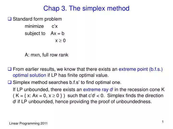
1. Chap 3. The simplex method • Standard form problem minimize c’x subject to Ax = b x  0 A: mxn, full row rank • From earlier results, we know that there exists an extreme point (b.f.s.) optimal solution if LP has finite optimal value. • Simplex method searches b.f.s’ to find optimal one. If LP unbounded, there exists an extreme ray di in the recession cone K ( K = { x: Ax = 0, x  0 } ) such that c’di < 0. Simplex finds the direction di if LP unbounded, hence providing the proof of unboundedness.

2. 3.1 Optimality conditions • A strategy for algorithm : Given a feasible solution x, look at the neighborhood of x for a feasible point that gives improved objective value. If no such point exists, we are at a local optimal point. In general such local optimal point is not global optimal. However, if we minimize a convex function over a convex set (convex program), local min is a global min point, which is the case for linear programming problem. (HW) • Def: P is polyhedron. x  P, d Rn is a feasible direction at x if   > 0 such that x + d  P • Given a b.f.s. x  P, ( xB = B-1b, xN = 0 for N: nonbasic) ( B = [ AB(1), AB(2), … , AB(m) ] ) want to find a new point x + d such that it satisfies Ax = b and x  0 and the new point gives an improved objective value.

3. Consider moving to x + d = where dj = 1 for some nonbasic variable xj 0 for other nonbasic variables except xj and xB xB + dB We require A(x + d) = b for  > 0  need Ad = 0 (iff condition to satisfy A(x + d) = b, for  > 0)  0 = Ad = i=1n Aidi = i = 1m AB(i)dB(i) + Aj = BdB + Aj  dB = -B-1Aj Assuming that columns of A are permuted so that A = [ B, N ] and x = (xB, xN), d = (dB, dN), d = is called j-th basic direction.

4. Note that  (n – m) basic directions when B is given. Recall {d : Ad = 0 } is the null space of A and its basis is given by columns of , where P is a permutation matrix for AP = [ B, N ] Each column here gives a basic direction. • Those n – m basic directions constitute a basis for null space of A (from earlier). Hence we can move along any direction d which is a linear combination of these basis vectors while satisfying A(x + d) = b,  > 0.

5. However, we also need to satisfy the nonnegativity constraints in addition to Ax = b to remain feasible. • Since dj = 1 > 0 for nonbasic variable index j and xj = 0 at the current solution, moving along (- dj ) will make xj  0 violated immediately. Hence we do not consider moving along -dj direction. Therefore, the direction we can move is the nonnegative linear combination of the basic directions, which is the cone generated by the n – m basic directions. Note that if a basic direction satisfies dB = -B-1Aj  0, it is an extreme ray of recession cone of P (recall HW). • In simplex method, we choose one basic direction as the direction of movement.

6. Two cases: (a) current solution x is nondegenerate : xB > 0 guarantees that xB + dB > 0 for some  > 0 (b) x is degenerate : some basic variable xB(i) = 0. It may happen that i-th component of dB = -B-1Aj is negative  Then xB(i) becomes negative if we move along d. So we cannot make  > 0. Details later.

7. x3 = 0 Figure 3.2: n = 5, n – m = 2 x1, x3 nonbasic at E. x3, x5 nonbasic at F (x4 basic at 0). F E x5 = 0 x1 = 0 x4 = 0 G x2 = 0

8. Now consider the cost function: Want to choose the direction that improves objective value ( c’(x + dj) – c’x = c’dj < 0 ) c’dj = (cB’, cN’)= cj – cB’B-1Aj  (reduced cost) If < 0, then objective value improves if we move to x + dj • Note) For i-th basic variable, may be computed using above formula.

9. Thm 3.1: (optimality condition) Consider b.f.s. x with basis matrix B. be the reduced cost vector. (a) If  0  x is optimal (sufficient condition for opt) (b) x is optimal and nondegenerate   0 Pf) (a) assume  0. y is an arbitrary point in P. Let d = y – x  Ad = 0  BdB + iN Aidi = 0  dB = - iN B-1Aidi c’d = c’y – c’x = cB’dB + iNcidi = iN (ci – cB’B-1Ai)di = ( , di  0 since yi  0, xi = 0 for i N and d = y – x )

10. (Pf-continued) ( Also may prove by contraposition: If x not optimal,  y = x + d s.t. c’y < c’x (note P is convex) Feasible direction d at x is in the cone generated by basic directions. Hence c’y – c’x = c’d = c’(i idi)< 0 , i  0  for some basic direction dj, c’dj= (cB, cN)(-B-1Aj, ej)’ = cj – cB‘B-1Aj < 0 ) (b) Suppose x is nondegenerate b.f.s. and for some j. xj must be a nonbasic variable and we can obtain improved solution by moving to x + dj ,  > 0 and small. Hence x is not optimal. 

11. Note that the condition c 0 is a sufficient condition for optimality of a b.f.s. x, but it is not necessary. The necessity holds only when x is nondegenerate. • Def 3.3: Basis matrix B is said to be optimal if

12. 3.2 Development of the simplex method • (Assume nondegenerate b.f.s. for the time being) Suppose we are at a b.f.s. x and computed , jN If  0,  j N, current solution is optimal. Otherwise, choose j  N such that < 0 and find d vector ( dj = 1, di = 0 for i  B(1), … , B(m), j, and dB = -B-1Aj ) Want to find * = max {   0 : x + d P }. Cost change is *c’d = * The vector d satisfies A(x + d) = b, also want to satisfy (x + d)  0

13. (a) If d  0, then (x + d)  0 for all   0 . Hence * =  (b) If di < 0 for some i, (xi + di )  0    - xi / di For nonbasic variables, di  0. Hence only consider basic variables Let y = x + *d. Have yj = * > 0 for entering nonbasic variable xj. (we assumed nondegeneracy, hence xB(i) > 0 for all basic variables) Let l be the index of the basic variable selected in the minimum ratio test, i.e.

14. Replace xB(l) in the basis with the entering variable xj. New basis matrix is Also replace the set { B(1), … , B(m) } of basic indices by { B(1), … , B(m) } given by B(i) = B(i), i  l, j, i = l

15. Thm 3.2: (a) AB(i) , i  l, and Aj are linearly independent. Hence is a basis matrix. (b) y = x + *d is a b.f.s. with basis Pf)

16. Pf-continue) (b) Have y  0, Ay = b, yi = 0, Columns of B linearly independent. Hence b.f.s.  • See the text for a complete description of an iteration of the simplex method. • Thm 3.3: Assume standard polyhedron P   and every b.f.s. is nondegenerate. Then simplex method terminates after a finite number of iterations. At termination, two possibilities: (a) optimal basis B and optimal b.f.s (b) Have found a vector d satisfying Ad = 0, d  0, and c’d < 0, and the optimal cost is - .

17. Remarks • 1) Suppose x nondegenerate b.f.s. and we move to x + d,  > 0 Consider the point y = x + *d, * > 0 and y feasible (nondegeneracy of x guarantees the existence of * > 0 and y feasible) Then A( x + *d ) = b y = ( yB , yN )  yB = xB + *dB > 0 for sufficiently small * > 0 yN = xN + *dN = 0 + *ej = (0, …, *, 0, …, 0) Since ( n – m – 1 ) of constraints xj  0 are active and m constraints Ax = b active, we have ( n – 1 ) constraints are active at ( x + *d ) (also the active constraints are lin. Ind.) and no more inequalities are active.

18. (continued) Hence y is in the face defined by the active constraints, which is one-dimensional since the equality set of the face is ( n – 1 )-dimensional. So y is in one-dimensional face of P (edge) and no other proper face of it. When * is such that at least one of the basic variable becomes 0 (say xl ), then entering nonbasic variable replaces xl in the basis and the new basis matrix is nonsingular and the leaving basic variable xl = 0  xl  0 becomes active. Hence we get a new b.f.s., which is a 0-dimensional face of P. For nondegenerate simplex iteration, we start from a b.f.s. ( 0-dim face), then follow an edge ( 1-dim face ) of P until we reach another b.f.s. ( 0-dim face)

19. (continued) The recession cone of P is K = { y : Ay = 0, y  0 } ( P = K + Q). Since d  K and ( n – 1 ) independent rows active at d, d is an extreme ray of K (recall HW) and c’d = cj – cB’B-1Aj < 0  LP unbounded. Hence, given a basis (b.f.s.), finding an extreme ray d (basic direction) in the recession cone with c’d < 0 provides a proof of unboundedness of LP.

20. Simplex method for degenerate problems • If degeneracy allowed, two possibilities : (a) current b.f.s. degenerate  * may be 0 (if, for some l, xB(l) = 0 and dB(l) < 0 ) Perform the iteration as usual with * = 0 New basis B is still nonsingular ( solution not changed, only basis changes), hence the current solution is b.f.s with different basis B. ( Note that we may have nondegenerate iteration although we have a degenerate solution.) (b) although * may be positive, new point may have more than one of the original basic variables become 0 at the new point. Only one of them exits the basis and the resulting solution is degenerate. (It happens when we have ties in the minimum ratio test.)

21. -g x Figure 3.3: n – m = 2. x4, x5 nonbasic. (g, f are basic dir.) Then pivot with x4 entering, x6 exiting basis. (h, -g are basic dir) Now if x5 enters basis, we follow the direction h until x1 0 becomes active, in which case x1 leaves basis. g f x5 = 0 x4 = 0 h x3 = 0 x6 = 0 y x2 = 0 x1 = 0

22. Cycling : a sequence of basis changes that leads back to the initial basis. ( only basis changes, no solution change) • Cycling may occur if there exists degeneracy. Finite termination of the simplex method is not guaranteed. Need special rules for entering and/or leaving variable selection to avoid cycling (later). • Although cycling hardly occurs in practice, prolonged degenerate iterations might happen frequently, especially in well-structured problems. Hence how to get out of degenerate iterations as early as possible is of practical concern.

23. Pivot Selection • (a) Smallest (largest) coefficient rule : choose xj with argminjN { cj : cj < 0 } • (b) largest increase rule : xj with cj < 0 and * | cj | is max. • (c) steepest edge rule • (d) maintain candidate list • (e) smallest subscript rule ( avoid cycling).

24. Review of calculus • Purpose: Interpret the value c’d in a different way and derive the logic for the steepest edge rule • Def: p > 0 integer. h : Rn R, then h(x)  o( ||x||p) if and only if limxk 0 h(xk)/ ||xk ||p = 0 for all sequences { xk } with xk 0 for all k, that converges to 0. • Def: f : Rn R is called differentiable at x iff there exists a vector f(x) (called gradient) such that f(z) = f(x) + f(x)’( z – x ) + o( ||z – x || ) or in other words, lim z  x { f(z) – f(x) - f(x)’( z – x )} / || z – x || = 0 (Frechet differentiability)

25. Def :f : Rn R. One sided directional derivative of f at x with respect to a vector y is defined as f’( x; y )  lim 0 { f(x+ y) – f(x) } /  if it exists. • Note that - f’( x; -y) = lim 0 { f(x+ y) – f(x) } /  . Hence the one-sided directional derivative f’( x; y) is two-sided iff f’( x; -y) exists and f’( x; -y) = -f’( x; y) • Def :i-th partial derivative of f at x : f(x)/xi = lim  0 { f( x+ei ) – f(x) }/ if it exists (two sided) ( Gateuax differentiability ) ( f is called Gateaux differentiable at x if all directional derivatives of f at a vector x exist and f’( x; y) is a linear function of y. F differentiability implies G differentiability, but not conversely. We do not need to distinguish F and G differentiability for our purposes here.)

26. Suppose f is F differentiable at x, then for any y  0 Hence f’( x; y) exists and f’( x; y) = f(x)’y (linear function of y) If f is F differentiable, then it implies f’( x; -y) = -f’( x; y) from above, hence f’( x; y) is two-sided. In particular,

27. In simplex algorithm, moving direction d = for xj entering. Then • Hence the rate of change c’d in the objective function when move in the direction d from x is the directional derivative. So cj – cB’B-1Aj is the rate of change of f when we move in the direction d. But, f’(x; d) is sensitive to the size (norm) of d. ( f’( x; kd) = f(x)(kd) = k f’( x; d) ) To make fair comparison among basic directions, use normalized vector d / ||d|| to compute f’( x; d)

28. Hence, among basic directions with cj < 0, choose the one with smallest normalized directional derivative. (steepest edge rule) • Problem here is that we need to compute ||dj|| (additional efforts needed). But, once ||dj|| is computed, it can be updated efficiently in subsequent iterations. Competitive (especially the dual form) against other rules in real implementation.