Download
1 / 40
400 likes | 525 Views
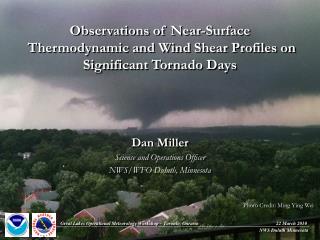
Observations of Near-Surface Thermodynamic and Wind Shear Profiles on Significant Tornado Days. Dan Miller Science and Operations Officer NWS/WFO Duluth, Minnesota. Photo Credit: Ming Ying Wei. Great Lakes Operational Meteorology Workshop – Toronto, Onrario. 22 March 2010.

E N D
Observations of Near-Surface Thermodynamic and Wind Shear Profiles on Significant Tornado Days Dan Miller Science and Operations Officer NWS/WFO Duluth, Minnesota Photo Credit: Ming Ying Wei Great Lakes Operational Meteorology Workshop – Toronto, Onrario 22 March 2010 NWS Duluth Minnesota
Some Preliminary Thoughts… • Compilation of case observations/discussions • There are more questions posed than conclusions drawn from this talk • Evidence warrants further investigation by researchers of these topics through modeling/field ops/etc. • The soundings/hodographs to be presented are in no way to be interpreted in a universal manner for forecasting significant tornado environments!
Multiple Cyclic Tornadic Supercells F2-F3 tornadoes Lots of 2-3” Hail Limited Wind no Tornadoes Which VWP/Hodo is “Better” for Tornadoes?
Lots of Hail/Wind 2 short-lived weak Tornadoes HP Supercells (strong cold pools) Multiple long-tracked F3-F5 tornadoes Classic Supercells Which Sounding is “Better” for Tornadoes?
Oklahoma: 3 May 1999 350 m agl wind 165 @41kt 1000 m agl SFC Wind 160 @17kt 1000 m agl Observed Storm Motion 350 m agl 00 UTC 1999 0504
Missouri: 4 May 2003 350 m agl wind 175 @24kt 1000 m agl Observed Storm Motion SFC Wind 150 @12kt 1000 m agl 350 m agl 00 UTC 2004 0503
Northeast Kansas: 4 May 2003 360 m agl wind 180 @35kt 1000 m agl Observed Storm Motion SFC Wind 165 @15kt 1000 m agl 360 m agl 18 UTC 2003 0504
Oklahoma: 8 May 2003 350 m agl wind 170 @34kt 1000 m agl SFC Wind 160 @13kt Observed Storm Motion 1000 m agl 350 m agl 00 UTC 2003 0509
Kansas/Oklahoma: 26 April 1991 350 m agl wind 165 @32kt 1000 m agl SFC Wind 178 @12kt 1000 m agl Observed Storm Motion 300 m agl 00 UTC 1991 0427
Ohio/Tennessee: 10 November 2002 400 m agl wind 195 @49kt 1000 m agl SFC Wind 180 @17kt Observed Storm Motion 1000 m agl 400 m agl 00 UTC 2002 1111
Pennsylvania/Ontario: 31 May 1985 400 m agl wind 200 @32kt 1000 m agl SFC Wind 195 @15kt Observed Storm Motion 1000 m agl 400 m agl 00 UTC 1985 0601
Ohio Valley Region: 3 April 1974 400 m agl wind 200 @38kt 1000 m agl Observed Storm Motion SFC Wind 185 @15kt 1000 m agl 400 m agl 00 UTC 1974 0404
Western Tennessee: 2 April 2006 500 m agl wind 225 @35kt 1000 m agl SFC Wind 207 @16kt Observed Storm Motion 1000 m agl 500 m agl 00 UTC 2006 0403
Minnesota: 16 June 1992 1000 m agl 350 m agl wind 100 @32kt Observed Storm Motion SFC Wind 095 @17kt 1000 m agl 350 m agl 00 UTC 1992 0617
Edmonton Alberta: 31 July 1987 1000 m agl Observed Storm Motion 1000 m agl 450 m agl wind 081 @18kt SFC Wind 070 @09kt 450 m agl 00 UTC 1987 0801
California (Sacramento) – 21 February 2005 Observed Storm Motion 1000 m agl 1000 m agl 500 m agl wind 070 @18kt SFC Wind 340 @10kt 500 m agl 21 UTC 2005 0221
Question:Is the “sickle” shape to the hodograph real, or merely an artifact of data sampling? Wind Measured By Radiosonde Surface wind measured by Anemometer Observed hodograph
Question:Is the “sickle” shape to the hodograph real, or merely an artifact of data sampling? 1000 m agl 190 @18kt 400 m agl wind 135 @18kt SFC Wind 125 @10kt NAM bufr forecast hodograph
Question:Is the “sickle” shape to the hodograph real, or merely an artifact of data sampling? ~350 m agl 55-60kt outbound ~350 m agl 60-65kt inbound Greensburg KS Event: 5/4/2007
Mean Parameters of the 20 Cases: (2/21/2005 Sacramento Case Not Included) Surface Temperature: 76 Surface Dewpoint: 68 Surface T/Td spread: 7.7 Surface Relative Humidity 69% LCL Height (agl):2630 ft (802 m) LFC Height (agl):4425 ft (1349 m) CAPE (surface parcel): 3206 j/kg CIN (surface parcel): 34 j/kg
Operational Implications? From Nordin and Brooks, 2002 How often do you get a warm and very humid airmass, that possesses strong instability and sufficient deep-layer shear for supercells that is also co-located with strong near-surface shear – and is nearly un-capped?
Some Important (and Perhaps Troublesome) Questions: 1) What do we mean when we say “elevated” vs. “surface-based” convection? 2) Do we need to consider “elevated” vs. “boundary-layer” vs. “surface- based” convection? 3) How do we *know* what parcels are ascending into the updraft? 4) What implications does this have for many of our near-storm environment forecast parameters?
All of this critical “stuff” is going on in a VERY shallow near-surface layer Now The Dirty Details: Red = SFC – 400m agl Cyan = 400m – 1000m agl Lavender = 1000m – 7000 m agl
457 m 1500 ft 553 m 1815 ft Just Exactly How Shallow is this Layer?
Surface-1 km shear vector Surface-400m shear vector Question:Is there a more effective way to examine low-level wind shear? Are We Looking Low Enough?
Mean Parameters of the 20 Cases: (2/21/2005 Sacramento Case Not Included) Height of hodograph kink agl: 399 m Bulk Shear Vector Magnitude (sfc-kink): 18 kt Bulk Shear Vector Magnitude (sfc-1 km): 25 kt Bulk Shear Vector Ratio: 0.72
Central Florida – 25 December 2006 1000 m agl 300 m agl wind 175 @39kt Observed Storm Motion SFC Wind 175 @12kt 1000 m agl 300 m agl 12 UTC 2006 1225
Question:What is our true skill in choosing the “correct” parcel to lift in the calculation of numerous popular near-storm environment parameters and indices?
Question:What is our true skill in choosing the “correct” parcel to lift in the calculation of numerous popular near-storm environment parameters and indices? What about the mixed boundary layer?
Question:Do we need to re-evaluate our use of the terms “elevated” and “surface-based” convection?
Question:Do we need to re-evaluate our use of the terms “elevated” and “surface-based” convection? Theta-e decreases rapidly with height What are the “correct” parcels with this thermodynamic profile? How do we define “surface-based” DMC?
How does the atmosphere produce/maintain this thermodynamic profile in the near-surface layer near max heating time? Question:What is the importance of surface heating in the contribution to instability on significant tornado days?
Question:Can we improve on the utility of the two near-storm environment significant tornado parameters that have shown the most promise: namely surface-1km EHI and surface-3km VGP? Calculation of both of these indices for some useful purpose requires an accurate input value of total CAPE and shear over the appropriate layer (0-1 km/0-3 km/etc.)… …but how do we know what is the appropriate parcel to choose for an accurate value of CAPE? – and therefore… …how do we know what effective shear the storm is tapping?
Implications for NSE Parameters: 100 mb Mean-Layer CAPE (MLCAPE) 100 mb Mean-Layer CIN (MLCIN) Lowest 100 mb Lowest 100 mb Averaging is “safer” - well-mixed BL should have uniform thetae Averaging is dangerous!! - thetae decreases rapidly with height in BL Difference in computed CAPE can be large - ~1000-2000 j/kg! **(VGP/EHI)** Difference in computed CAPE is small
Implications for NSE Parameters: 0-1 km and 0-3 km Energy-Helicity Index (EHI) 0-3 km Vorticity Generation Potential (VGP) If the storm isn’t tapping *surface* parcels (i.e. below ~400-500m) – it isn’t realizing the full effect of the calculated EHI or VGP! Lowest 100 mb Might this explain in part why VGP in particular is plagued by high false alarm ratios (>80%)?
Question:If a systematic search of the historical upper air database was performed, would a superposition of low-level shear and thermodynamic profiles presented here be present in a majority of significant tornado events? Question:Would a systematic search of the historical upper air database also identify null cases?
Final Thought... Superposition of these profiles appears to be critical – NOT only the “sickle” hodograph Red = SFC – 400m agl Cyan = 400m – 1000m agl Lavender = 1000m – 7000 m agl
Acknowledgements David Andra: NWS/WFO Norman OK Michael Foster: NWS/WFO Norman OK Rich Thompson: NWS/SPC Norman OK Dr. Bob Conzemius: WindLogics Grand Rapids MN Dr. Bruce Lee: WindLogics Grand Rapids MN Doug Speheger: NWS/WFO Norman OK Kevin Scharfenberg: NSSL Norman OK Bob Johns: former SOO SPC Norman OK Jon Davies: Private Meteorologist Kansas City MO Todd Lindley: NWS/WFO Lubbock TX Dr. Chris Weiss: Texas Tech University Lubbock TX Dr. Matt Bunkers: NWS/WFO Rapid City SD Dr. David Blanchard: NWS/WFO Flagstaff AZ
Thanks for your attention! Questions? Photo Credit: Todd Lindley