Download
1 / 30
300 likes | 471 Views
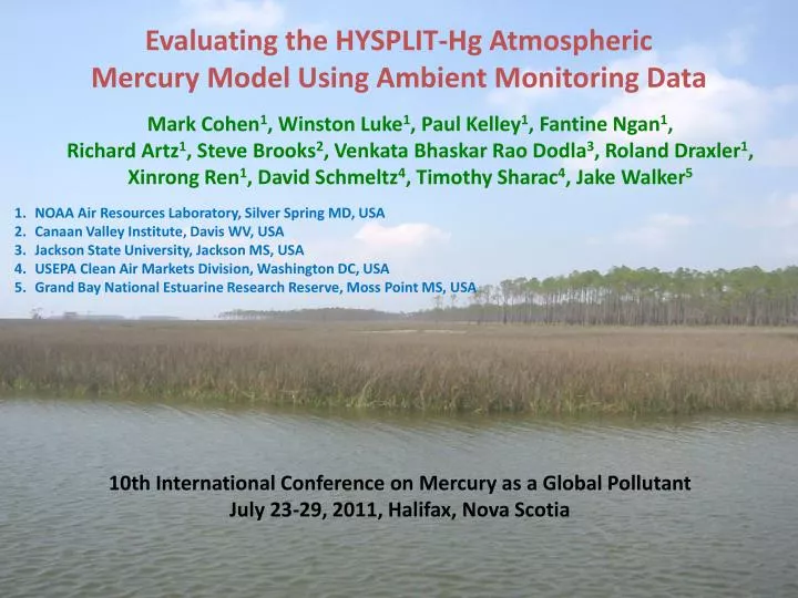
Evaluating the HYSPLIT-Hg Atmospheric Mercury Model Using Ambient Monitoring Data. Mark Cohen 1 , Winston Luke 1 , Paul Kelley 1 , Fantine Ngan 1 , Richard Artz 1 , Steve Brooks 2 , Venkata Bhaskar Rao Dodla 3 , Roland Draxler 1 ,

E N D
Evaluating the HYSPLIT-Hg Atmospheric Mercury Model Using Ambient Monitoring Data Mark Cohen1, Winston Luke1, Paul Kelley1, Fantine Ngan1, Richard Artz1, Steve Brooks2, VenkataBhaskarRao Dodla3, Roland Draxler1, Xinrong Ren1, David Schmeltz4, Timothy Sharac4, Jake Walker5 NOAA Air Resources Laboratory, Silver Spring MD, USA Canaan Valley Institute, Davis WV, USA Jackson State University, Jackson MS, USA USEPA Clean Air Markets Division, Washington DC, USA Grand Bay National Estuarine Research Reserve, Moss Point MS, USA 10th International Conference on Mercury as a Global Pollutant July 23-29, 2011, Halifax, Nova Scotia
NOAA Air Resources Laboratory: Five Collaborative Speciated Atmospheric Mercury Measurement Sites Emissions (kg/yr) Allegheny Portage 5-10 10-50 50-100 100–300 300–500 Mauna Loa 500–1000 1000–3500 Beltsville Canaan Valley Type of Emissions Source coal-fired power plants other fuel combustion waste incineration metallurgical Grand Bay NERR manufacturing & other 2002 mercury emissions sources based on data from USEPA, Envr. Canada and the CEC
Atmospheric Mercury Monitoring Station at the Grand Bay NERR precipitation collection mercury and trace gas monitoring tower (10 meters) Mercury Deposition Network and heavy metals precipitation amount major ions (“acid rain”)
Oct Nov Dec Jan Feb Mar Apr May Jun Jul Aug Sep time series of RGM concentrations measured at Grand Bay May 5-6 2008 episode Then down for ~2 months due to hurricanes …. …. 2007 2008
two co-located speciated mercury measurement suites provide continuous “coverage” and allow peaks to be verified Date
Can we reproduce this episode with an atmospheric mercury model? Hg from other sources: local, regional & more distant • Peaks are important to understand • Opportunity for model evaluation • Just one episode of many emissions of Hg(0), Hg(II), Hg(p) Measurement of ambient air concentrations Measurement of wet deposition
Mississippi Alabama Greene size/shape of symbol denotes amount of Reactive Gaseous Mercury (RGM) emitted during 2002 (kg/yr) Ipsco Steel: significant mercury emissions in 2002 NEI, but negligible emissions reported in 2008 TRI Brewton Paper Mill: no emissions according to 2002-2008 Toxic Release Inventory Lowman: big reduction in Hg emissions reported in 2008 5 - 10 10 - 50 50 - 100 100 – 300 Lowman color of symbol denotes type of mercury source Morrow coal-fired power plants Barry other fuel combustion waste incineration Florida Mobile* metallurgical Crist manufacturing & other Daniel Louisiana Watson urban areas Pascagoula Waste Incinerator: in 2002 NEI but shut down in 2001 Grand Bay site * Also called “Kimberly Clark Paper”
NOAA “EDAS 40km” met data (grid points shown here) • Ok for regional analysis, but too coarse for local analysis • Unlikely to simulate sea-breeze well, and in general, wind speed and wind direction are unlikely to be very accurate on local scales Grand Bay site
We created a 4km resolution met data set – also with enhanced vertical resolution – using the Weather Research and Forecasting (WRF) model (grid points shown here)
May 5 May 6 May 7 May 3 May 4 Mercury peaks Model over-predicted wind speed Measurements at the Grand Bay NERR site * Model: WRF(a) (NOAH Land Surface Model + nudging) Model: WRF(b) (PX Land Surface Model + nudging)
May 5 May 6 May 7 May 3 May 4 Modeled wind did not turn to north Mercury peaks Measurements at the Grand Bay NERR site * Model: WRF(a) (NOAH Land Surface Model + nudging) Model: WRF(b) (PX Land Surface Model + nudging)
This is the period that you just saw – a measured peak, but not a modeled peak (BARRY - blue line) RGM Measurements #1 #2 BARRY DANIEL One set of model results CRIST GREENE LOWMAN WATSON MOBILE
We typically assume emissions are constant throughout the year • May 2008: “typical” month for SO2 emissions at the Daniel plant May 2008 Source of data:USEPA Clean Air Markets Division
But, hourly SO2 emissions at the Daniel plant were not constant… and so Hg emissions were also likely variable May 4-7, 2008 Source of data:USEPA Clean Air Markets Division
SOME CONCLUDING THOUGHTS (and questions): • In order to “use” the AMNet data, we need • Emissions information with higher temporal resolution (better than annual once every 3 years) • Meteorological data with higher resolution • …no matter what kind of analyses we are doing • Comparing Trends; Trajectories; Dispersion • Justification for the network depends on being able to use the data meaningfully! • How can we improve this situation?
This model evaluation exercise will be more fully characterized for this one episode at this one site • Of course, must look at other episodes, other sites • Variations and uncertainties in meteorology and emissions make local plumes “stochastic”… • Even if a model was “perfect” it would not be generally possible to reproduce a local plume hit at a monitoring site. • What is the best way to evaluate (and improve) models?
EXTRA SLIDES
Modeling – Comprehensive Fate and Transport Simulations • Start with an emissions inventory • Use gridded meteorological data • Simulate the dispersion, chemical transformation, and wet and dry deposition of mercury emitted to the air • Source-attribution information needed at the end, so optimize modeling system and approach to allow source-receptor information to be captured • HYSPLIT-Hg developed over the last ~10 years with specialized algorithms for simulation of atmospheric mercury
(Proposed Alternative) Figure 3. Time series of Reactive Gaseous Mercury (RGM), Fine Particulate Mercury (FPM) and Gaseous Elemental Mercury (GEM) from two co-located instruments (D1 and D2) (top graph) and of SO2, O3, NO, NOy, and CO (bottom graph) measured at the Grand Bay NERR from May 3-8, 2008