Download
1 / 36
360 likes | 639 Views
Monopoly. Monopoly: Why?. Natural monopoly (increasing returns to scale), e.g. (parts of) utility companies? Artificial monopoly a patent; e.g. a new drug sole ownership of a resource; e.g. a toll bridge formation of a cartel; e.g. OPEC. Monopoly: Assumptions. Many buyers

E N D
Monopoly: Why? • Natural monopoly (increasing returns to scale), e.g. (parts of) utility companies? • Artificial monopoly • a patent; e.g. a new drug • sole ownership of a resource; e.g. a toll bridge • formation of a cartel; e.g. OPEC
Monopoly: Assumptions • Many buyers • Only one seller i.e. not a price-taker • (Homogeneous product) • Perfect information • Restricted entry (and possibly exit)
Monopoly: Features • The monopolist’s demand curve is the (downward sloping) market demand curve • The monopolist can alter the market price by adjusting its output level.
Monopoly: Market Behaviour p(y) Higher output y causes alower market price, p(y). D y = Q
Monopoly: Market Behaviour Suppose that the monopolist seeks to maximize economic profit What output level y* maximizes profit?
Monopoly: Market Behaviour At the profit-maximizing output level, the slopes of the revenue and total cost curves are equal, i.e. MR(y*) = MC(y*)
Marginal Revenue: Example p = a – by (inverse demand curve) TR = py (total revenue) TR = ay - by2 Therefore, MR(y) = a - 2by < a - by = p for y > 0
Marginal Revenue: Example MR= a - 2by < a - by = p for y > 0 P P = a - by a a/b y a/2b MR = a - 2by
Monopoly: Market Behaviour The aim is to maximise profits MC = MR < 0 MR lies inside/below the demand curve Note: Contrast with perfect competition (MR = P)
Monopoly: Equilibrium P Demand y = Q MR
Monopoly: Equilibrium MC P y Demand MR
Monopoly: Equilibrium MC P AC y Demand MR
Monopoly: Equilibrium MC Output Decision MC = MR P AC ym y Demand MR
Monopoly: Equilibrium MC Pm = the price P AC Pm ym y Demand MR
Monopoly: Equilibrium • Firm = Market • Short run equilibrium diagram = long run equilibrium diagram (apart from shape of cost curves) • At qm: pm > AC therefore you have excess (abnormal, supernormal) profits • Short run losses are also possible
Monopoly: Equilibrium MC The shaded area is the excess profit P AC Pm ym y Demand MR
Monopoly: Elasticity WHY? Increasing output by y will have two effects on profits • When the monopoly sells more output, its revenue increase by py • The monopolist receives a lower price for all of its output
Monopoly: Elasticity Rearranging we get the change in revenue when output changes i.e. MR
Monopoly: Elasticity = elasticity of demand
Monopoly: Elasticity Recall MR = MC, therefore, Therefore, in the case of monopoly, < -1, i.e. || 1. The monopolist produces on the elastic part of the demand curve.
Application: Tax Incidence in Monopoly MC curve is assumed to be constant (for ease of analysis) P MC y Demand MR
Application: Tax Incidence in Monopoly • Claim When you have a linear demand curve, a constant marginal cost curve and a tax is introduced, price to consumers increases by “only” 50% of the tax, i.e. “only” 50% of the tax is passed on to consumers
Application: Tax Incidence in Monopoly Output decision is as before, i.e. MC=MR So Ybt is the output before the tax is imposed P MCbt ybt y Demand MR
Application: Tax Incidence in Monopoly Price is also the same as before Pbt = price before tax is introduced. P Pbt MCbt ybt y Demand MR
Application: Tax Incidence in Monopoly The tax causes the MC curve to shift upwards P Pbt MCat MCbt ybt y Demand MR
Application: Tax Incidence in Monopoly The tax will cause the MC curve to shift upwards. P Pbt MCat MCbt ybt y Demand MR
Application: Tax Incidence in Monopoly Price post tax is at Ppt and it higher than before. P Ppt Pbt MCat MCbt ybt yat y Demand MR
Application: Tax Incidence in MonopolyFormal Proof Step 1: Define the linear (inverse) demand curve Step 2: Assume marginal costs are constant MC = C Step 3: Profit is equal to total revenue minus total cost
Application: Tax Incidence in MonopolyFormal Proof Step 4: Rewrite the profit equation as Step 5 : Replace price with P=a-bY Profit is now a function of output only
Application: Tax Incidence in MonopolyFormal Proof Step 6: Simplify Step 7: Maximise profits by differentiating profit with respect to output and setting equal to zero
Application: Tax Incidence in MonopolyFormal Proof Step 8: Solve for the profit maximising level of output (Ybt)
Application: Tax Incidence in MonopolyFormal Proof Step 9: Solve for the price (Pbt) by substituting Ybt into the (inverse) demand function Recall that P = a - bY therefore
Application: Tax Incidence in MonopolyFormal Proof Step 10: Simplify Multiply by - b b cancels out
Application: Tax Incidence in MonopolyFormal Proof Step 11: Replace C = MC with C = MC + t (one could repeat all of the above algebra if unconvinced) Price before tax So price after the tax Pat increases by t/2