Download
1 / 71
720 likes | 770 Views
Learn about descriptive and inferential statistics, measures of center (mean, median, mode), variation, and exploring data. Understand skewness, standard deviation, and range.

E N D
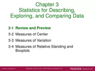
Chapter 3Statistics for Describing, Exploring, and Comparing Data 3-1 Overview 3-2 Measures of Center 3-3 Measures of Variation 3-4 Measures of Relative Standing 3-5 Exploratory Data Analysis (EDA)
Section 3-1 Overview Created by Tom Wegleitner, Centreville, Virginia
Descriptive Statistics summarize or describethe important characteristics of a known set of data Inferential Statistics use sample data to makeinferences (or generalizations)about a population Overview
Section 3-2 Measures of Center Created by Tom Wegleitner, Centreville, Virginia
Key Concept When describing, exploring, and comparing data sets, these characteristics are usually extremely important: center, variation, distribution, outliers, and changes over time.
Definition • Measure of Center • the value at the center or middle of a data set
Arithmetic Mean (Mean) the measure of center obtained by adding the values and dividing the total by the number of values Definition
denotes the sum of a set of values. x is the variable usually used to represent the individual data values. n represents the number of values in a sample. N represents the number of values in a population. Notation
µis pronounced ‘mu’ and denotes themean of all values in a population x x x = n x µ = N Notation is pronounced ‘x-bar’ and denotes the mean of a set of sample values
Median the middle value when the original data values are arranged in order of increasing (or decreasing) magnitude • often denoted by x (pronounced ‘x-tilde’) ~ Definitions • is not affected by an extreme value
Finding the Median • If the number of values is odd, the median is the number located in the exact middle of the list. • If the number of values is even, the median is found by computing the mean of the two middle numbers.
5.40 1.10 0.42 0.73 0.48 1.10 0.42 0.48 0.73 1.10 1.10 5.40 (in order - even number of values – no exact middle shared by two numbers) 0.73 + 1.10 MEDIAN is 0.915 2 5.40 1.10 0.42 0.73 0.48 1.10 0.66 0.42 0.48 0.66 0.73 1.10 1.10 5.40 (in order - odd number of values) exact middle MEDIANis 0.73
Mode the value that occurs most frequently Mode is not always unique A data set may be: Bimodal Multimodal No Mode Definitions Mode is the only measure of central tendency that can be used with nominal data
Mode is 1.10 Bimodal - 27 & 55 No Mode Mode - Examples a. 5.40 1.10 0.42 0.73 0.48 1.10 b. 27 27 27 55 55 55 88 88 99 c. 1 2 3 6 7 8 9 10
Midrange the value midway between the maximum and minimum values in the original data set maximum value + minimum value Midrange= 2 Definition
Carry one more decimal place than is present in the original set of values. Round-off Rule for Measures of Center
Assume that in each class, all sample values are equal to the class midpoint. Mean from a Frequency Distribution
use class midpoint of classes for variable x Mean from a Frequency Distribution
(w •x) x = w Weighted Mean In some cases, values vary in their degree of importance, so they are weighted accordingly.
Symmetric distribution of data is symmetric if the left half of its histogram is roughly a mirror image of its right half Skewed distribution of data is skewed if it is not symmetric and if it extends more to one side than the other Definitions
Recap In this section we have discussed: • Types of measures of center Mean Median Mode • Mean from a frequency distribution • Weighted means • Best measures of center • Skewness
Section 3-3 Measures of Variation Created by Tom Wegleitner, Centreville, Virginia
Key Concept Because this section introduces the concept of variation, which is something so important in statistics, this is one of the most important sections in the entire book. Place a high priority on how tointerpretvalues of standard deviation.
Therangeof a set of data is the difference between the maximum value and the minimum value. Definition Range = (maximum value) – (minimum value)
Definition Thestandard deviationof a set of sample values is a measure of variation of values about the mean.
(x - x)2 s= n -1 Sample Standard Deviation Formula
n(x2)- (x)2 s= n (n -1) Sample Standard Deviation (Shortcut Formula)
Standard Deviation - Important Properties • The standard deviation is a measure of variation of all values from the mean. • The value of the standard deviation s is usually positive. • The value of the standard deviation s can increase dramatically with the inclusion of one or more outliers (data values far away from all others). • The units of the standard deviation s are the same as the units of the original data values.
Population Standard Deviation (x - µ) 2 = N This formula is similar to the previous formula, but instead, the population mean and population size are used.
Population variance: Square of the population standard deviation Definition • The variance of a set of values is a measure of variation equal to the square of the standard deviation. • Sample variance: Square of the sample standard deviation s
Variance - Notation standard deviation squared s } 2 Sample variance Notation 2 Population variance
Carry one more decimal place than is present in the original set of data. Round-off Rulefor Measures of Variation Round only the final answer, not values in the middle of a calculation.
Range 4 s Estimation of Standard Deviation Range Rule of Thumb For estimating a value of the standard deviation s, Use Where range = (maximum value) – (minimum value)
= Minimum “usual” value (mean) – 2 X (standard deviation) = Maximum “usual” value (mean) + 2 X (standard deviation) Estimation of Standard Deviation Range Rule of Thumb For interpreting a known value of the standard deviation s,find rough estimates of the minimum and maximum “usual” sample values by using:
Definition Empirical (68-95-99.7) Rule For data sets having a distribution that is approximately bell shaped, the following properties apply: • About 68% of all values fall within 1 standard deviation of the mean. • About 95% of all values fall within 2 standard deviations of the mean. • About 99.7% of all values fall within 3 standard deviations of the mean.
Definition Chebyshev’s Theorem The proportion (or fraction) of any set of data lying within K standard deviations of the mean is always at least 1-1/K2, where K is any positive number greater than 1. • For K = 2, at least 3/4 (or 75%) of all values lie within 2 standard deviations of the mean. • For K = 3, at least 8/9 (or 89%) of all values lie within 3 standard deviations of the mean.
Rationale for using n-1 versus n The end of Section 3-3 has a detailed explanation of why n – 1 rather than n is used. The student should study it carefully.
s s · 100% · 100% CV = CV = m x Definition Thecoefficient of variation(or CV) for a set of sample or population data, expressed as a percent, describes the standard deviation relative to the mean. Sample Population
Recap In this section we have looked at: • Range • Standard deviation of a sample and population • Variance of a sample and population • Range rule of thumb • Empirical distribution • Chebyshev’s theorem • Coefficient of variation (CV)
Section 3-4 Measures of Relative Standing Created by Tom Wegleitner, Centreville, Virginia
Key Concept This section introduces measures that can be used to compare values from different data sets, or to compare values within the same data set. The most important of these is the concept of thez score.
z Score(or standardized value) the number of standard deviations that a given valuexis above or below the mean Definition
Sample Population x - µ x - x z = s z = Measures of Position z score Round z to 2 decimal places
Interpreting Z Scores Whenever a value is less than the mean, its corresponding z score is negative Ordinary values: z score between –2 and 2 Unusual Values: z score < -2 or z score > 2
Definition • Q1 (First Quartile)separates the bottom 25% of sorted values from the top 75%. • Q2 (Second Quartile)same as the median; separates the bottom 50% of sorted values from the top 50%. • Q1 (Third Quartile)separates the bottom 75% of sorted values from the top 25%.