Download
1 / 25
250 likes | 439 Views
Workshop Agenda. Trajectory Computational Method. How is a trajectory calculated?

E N D
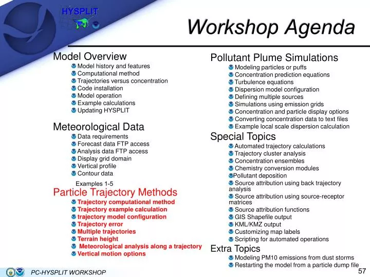
Workshop Agenda PC-HYSPLIT WORKSHOP
Trajectory Computational Method How is a trajectory calculated? If we assume that a particle passively follows the wind, then its trajectory is just the integration of the particle position vector in space and time. The final position is computed from the average velocity at the initial position (P) and first-guess position (P'). P'(t+ Δ t) = P(t) + V(P,t) Δt P(t+Δt) = P(t) + 0.5 [ V( P,t) + V(P',t+Δt) ] Δt The integration time step is variable:VmaxΔt < 0.75 meteo. grid spacing PC-HYSPLIT WORKSHOP
Trajectory Computational Method The meteorological data remain on the native horizontal coordinate system when read by HYSPLIT, but are interpolated to an internal terrain-following (σ) vertical coordinate system during computation: σ = ( Ztop – Zmsl ) / ( Ztop – Zgl ) Ztop - top of the trajectory model’s coordinate systemZgl - height of the ground levelZmsl - height of the internal coordinate The model’s internal heights can be chosen at any interval, however a quadratic relationship between height and model level is specified, such that each level’s height with respect to the model’s internal index, k, is defined by Zagl = ak2 + bk +c The constants are automatically defined such that the model’s internal resolution has the same or better vertical resolution than the input meteorological data. PC-HYSPLIT WORKSHOP
Trajectory Computational Method To illustrate this process, a simple forward trajectory was calculated with the NAM 40 km meteorological data from (60N, 110W) at 2500 m-agl for a total of 84 hours using the isobaric (constant pressure) vertical motion method, as shown below. The relationship of the trajectory to the temporal and spatial variations of the 700 hPA height field (approximate height of trajectory) is illustrated in the attached animation which was created using only the standard tools that come with PC HYSPLIT. PC-HYSPLIT WORKSHOP
Trajectory Model Configuration Now that you’ve had some time to practice running trajectories, a more thorough description of some of the GUI inputs will be presented. Starting Location Setup: A starting location(s) can be entered directly from this menu or a position may be chosen from a predefined list. This list is located in the working directory, is user editable, and named plants.txt. Heights are always entered as meters above ground level (agl). Top of the model (m agl): the height above which the meteorological data are not processed. For calculations within the troposphere, 10 km is a good value. Trajectories are terminated when they reach this height. Processing fewer levels reduces computational times. PC-HYSPLIT WORKSHOP
Trajectory Model Configuration One key feature for any simulation is selecting the best meteorological data. In the current version of HYSPLIT up to 12 meteorological files may be defined simultaneously. When multiple files are defined, at each integration step, the model uses the finest spatial resolution file at the location and time of the trajectory end-point. This can be useful if you have several higher resolution grids “nested” within each other. The Add Meteorology Files button is used to select multiple meteorological data files. The Clear button will erase all selected files from the list. In the example below, both the NAM 12 km and GFS latitude/longitude files have been selected for the next example. PC-HYSPLIT WORKSHOP
Trajectory Model Configuration For this example, an isobaric forward trajectory was started at 1200 UTC on December 19, 2005, from a height of 2.5 km at 46N, 68W. The total run time was set to 84 hours and both the NAMF12 and the GFSFLL meteorological data files were selected (previous slide). Execution of the CONTROL file for this case results in a trajectory (right) that goes northeast using the NAM 12 km forecast file until running off the NAM domain (~ 50N). The model then uses the GFS for the remainder of the calculation. The meteorological file identifier is written with each end-point position in the second column of the ASCII trajectory tdump output file. The diagnostic MESSAGE file also provides additional detail about the calculation. In this example the switch from NAM to GFS occurs at 0900 GMT on December 20, 2005, causing the 0900 and 1200 GMT data to be reloaded. PC-HYSPLIT WORKSHOP
Trajectory Error A common question often arises when running trajectories.... "What is the error associated with a given trajectory calculation." From the literature, one can estimate the total error to be anywhere from 15 to 30% of the travel distance. The total error is composed of four error components: • physical error due to the inadequacy of the data’s representation of the atmosphere in space and time, • computational error due to numerical inaccuracies, • measurementerrors in creating the model’s meteorological data fields, • forecast error if using forecast meteorology. Physical Error The physical component of the error is related to how well the numerical fields estimate the true flow field. There is no way of knowing this error without independent verification data. PC-HYSPLIT WORKSHOP
Trajectory Error The integration error component of computational error can be estimated by computing a backward trajectory from the forward trajectory endpoint. The error is then 1/2 the distance of the final endpoint from the starting point. In this example, the final endpoint position (67.574N, 26.813W, 2332.7 m AGL) from the previous tdumpendpoints file was used as the starting point (on the 23th 0000 UTC) for a backward trajectory calculation. When running this case, insure that the endpoints file names are different for both the forward and backward calculations by setting the tdump filename to tdumpback, for example. Computational Error The computational component of the error is composed of: • the integration error (part of which is due to truncation) and, • the data resolution error, i.e., trying to represent a continuous function, the atmospheric flow field, with gridded data points of limited resolution in space and time. PC-HYSPLIT WORKSHOP
Trajectory Error Integration Error To show the differences between the forward and backward trajectories, display both of them on the same plot by entering both file names in the Input endpoints: box of the Trajectory Display GUI using a + symbol (e.g. ./tdump+tdumpback). Note how the backward (blue) trajectory returns very close to the initial forward (red) starting location, indicating very little integrationerror. Most of the time the integrationerror is very small compared to resolutionerror. You can also see that the model automatically switched back to the NAM 12 km grid at 0800 UTC on December 20 by viewing the tdumpback endpoints file. PC-HYSPLIT WORKSHOP
Trajectory Error Resolution Error The resolution error component of computational error can be estimated by starting several trajectories about the initial point by offset ting them in the horizontal and vertical. The divergence of these trajectories will give an estimate of the uncertainty due to divergence in the flow field. An initial offset should be used that is comparable to the estimated integration error. In this example, there is little horizontal error, but vertical offset produces spread at later times. One component of the resolution error that is difficult to estimate relates to the size and speed of movement of various flow features through the grid. There should be a sufficient number of sampling points (in space and time) to avoid aliasing errors. Typically, a grid resolution of "x" can only represent wavelengths of "4x". This error will be a function of the meteorological conditions. PC-HYSPLIT WORKSHOP
Trajectory Error Another method of ascertaining the integration error is to run trajectories from the same location using several different sources of meteorological data. In this example (right), trajectories have been computed using meteorological data from NAM(12 km)/GFS (red), RUC/GFS (blue), and MM545/GFS (green). After the first 36 hours, differences between trajectories indicate that the integration error is much greater than the numerical error. Note that the green trajectory went up near the end because it hit Greenland (HYSPLIT is terrain following). These trajectories are more similar than most simulations due to the isobaric assumption that was made for this case. PC-HYSPLIT WORKSHOP
Multiple Trajectories Multiple Trajectories from same Location Trajectories can be started at regular time intervals from the same location by setting the restart interval to something other than 0 hrs. Clicking on the Advanced / Configuration Setup / Trajectory menu tab produces another menu (right) for entries to the optional trajectory namelist file SETUP.CFG used by the model for more options. Clicking on Multiple trajectories in time Menu button produces the menu shown to the right. To demonstrate the restart feature, change the Restart interval to 3 hrs, click Save, click Save again, and leave all other trajectory parameters the same as in the original 700 hPa isobaric trajectory previously computed at 46N, 68W.
Multiple Trajectories Multiple Trajectories from same Location (cont.) After clicking on Run Standard Model a message box (shown at right) will appear to indicate that a SETUP.CFG configuration file exists and ask if you want to run with it. In this case since we made changes to the advanced settings, choose Run with SETUP. The resulting trajectory graphic shows new trajectories every 3 hours, terminating at the end of the 84 h computational period. Trajectories starting after the initial time will have a shorter duration. All trajectories can be set to have the same duration from the Advanced menu tab.
Multiple Trajectories Trajectory Matrix (grid of starting locations) • The model supports an unlimited number of starting locations, however the GUI is limited by the user’s screen size (GUI will extend off the bottom with too many selections). • A matrix of starting locations can be defined by selecting three points, representing the lower left, upper right, and location increment from the Setup Starting Locations menu button (see example to the below). • Once configured, the Run Matrix option is selected through the Special Simulations menu tab of the Trajectory menu instead of Run Standard Model. • This causes the locations defined by the grid (in this case 25) to be calculated and written to the CONTROLfile. PC-HYSPLIT WORKSHOP
Multiple Trajectories Trajectory Matrix Example The resulting graphic should be similar to the one shown above; a matrix of 24-h duration isobaric trajectories. Again there is very little differences noted between the trajectories indicating small temporal and spatial differences in the meteorology in this region. Note that we are using spatial and temporal offsets to ascertain the trajectory error or in this case sensitivity to the meteorological data. • Rerun the 700 hPa isobaric case again but change the Total run time to 24 hours and choose the 3 source locations from the previous slide. • From the Advanced/Configuration Setup/Trajectory menu choose Define subgrid and MSL/AGL UNITS menu and set the height unit Relative to mean-sea-level because the terrain height varies across the matrix. Save. • Reset the Restart Interval back to 0. Save. • Save the advanced settings and run the Matrix from the Special Runs menu tab (run with SETUP). • When finished set the Time Label Interval (hrs) to 0 in the Trajectory Display GUI) before executing the display (this makes a less cluttered display) and the zoom to 80. PC-HYSPLIT WORKSHOP
Terrain Height • Trajectory starting height defaults to meters AGL (above ground level), but can be changed to meters MSL (above mean sea level) from the Advanced / Configuration Setup menu tab as was done in the previous exercise. • Regardless of how the input heights are defined, internally HYSPLIT treats all heights in a terrain following coordinate system based on the chosen meteorological data. • These heights may be quite different from the actual terrain height at a point of interest. • As an example, examine the various model estimated terrain heights (right) for Broomfield (KBJC), Colorado, at 39.92N and 105.12W, which has a surface height of 1724 m above MSL. PC-HYSPLIT WORKSHOP
Terrain Height The terrain heights for the NAM 12 km (left) and GFS (right) are shown below (Bloomfield is indicated by the black star). The terrain in the vicinity of Bloomfield is much smoother in the coarser GFS than the NAM and the terrain gradient is much steeper in the NAM and therefore we would expect to see differences in the terrains. Also, when the model terrain is consistently above the true terrain in all models, one might suspect that the station is located in a valley, as in this case. In this situation, all one can do is assume that true ground-level is at the model's terrain height and proceed with the realization that the lower levels of the flow field may at times be constrained in ways that are not evident in the coarser gridded meteorological data fields. NAM GFS PC-HYSPLIT WORKSHOP
Terrain Height • In the example to the right, we plotted 3 separate trajectory results on the same map using the NAM 12 km (blue), the MM5 45 km (green), and the 1 degree GFS (red) originating from 10 m above model ground level (AGL). • Even though all the trajectories start out at the same height AGL, they start at different pressure levels due to differences in elevation between the data various datasets. PC-HYSPLIT WORKSHOP
Meteorological Analysis Along a Trajectory • HYSPLIT can provide details on some of the meteorological parameters along the trajectory if the appropriate boxes are selected by the user in the Advanced/Configuration Setup/Trajectory menu. • This information can be useful in diagnosing why a trajectory took the path it did, to show the underlying terrain height, to show the mixed layer depth along the trajectory, or to show if any precipitation was being produced along the trajectory path by the meteorological model. • Currently only ambient and potential temperature, precipitation, mixing depth, relative humidity, solar radiation, and terrain height are available to output or display. • One or more meteorological fields may be selected and all will be written to the trajectory endpoints file in the columns to the right, however only the rightmost (or last selected) variable will be plotted at the bottom of the trajectory map if the plotting option is enabled. PC-HYSPLIT WORKSHOP
Meteorological Analysis Along a Trajectory Trajectory Example • Configure the model for a trajectory originating at Broomfield, Colorado, (39.92N and 105.12W) using the NAM 12 km data. • Set the starting height to 1500 m, • the vertical motion data field to 0 (Data), • and the total run time to 84 hours. • In the advanced trajectory menu click on Add METEOROLOGY output along trajectory • Choose Terrain Height (right) and Save. • Save the configuration and choose Run with SETUP. A flag is set in the SETUP.CFG when meteorological variables are selected. • In order to plot the terrain height along the trajectory in the vertical cross-section plot, choose Meters-agl as the vertical coordinate in the Trajectory Display menu. PC-HYSPLIT WORKSHOP
Meteorological Analysis Along a Trajectory • For the most part, the resulting trajectory (right) follows the terrain as the terrain descends from Colorado into Texas. • If you choose Pressure as the Vertical Coordinate, the trajectory may look like it is descending in height, but in reality it is following the descending terrain, so care must be exercised when interpreting the up or down movement of trajectories with respect to height above model ground level and pressure vertical height coordinates. • The terrain heights can be viewed as the right-most column of the trajectory endpoints file (tdump) PC-HYSPLIT WORKSHOP
Meteorological Analysis Along a Trajectory • Rerun the last case, but instead of Terrain Height, select Mixing Depth. • In order to display a meteorological variable other than Terrain Height, select Meteo-varb as the vertical coordinate in the Trajectory Display menu (upper-right). • This plot shows that the mixed layer depth along the trajectory varied from 250 m on the first day (HYSPLIT sets the lower depth to a minimum of 250 m) to 659 m during the afternoon of the 21st. PC-HYSPLIT WORKSHOP
Vertical Motion Options • There are six vertical motion options in PC-HYSPLIT. • The suggested default (0:data) uses the vertical velocity field included with most meteorological data. • Other options may be required for special situations such as following the transport of a balloon on a constant density surface, comparing isobaric flow fields between data sets, or situations when the meteorological data’s vertical velocity field may be too noisy compared with the time step at which the data are available (high spatial resolution simulations). • In the sigma option the trajectory remains on its original terrain following sigma surface. • In the isobaric, isentropic, and constant density (isopycnic) options, the vertical velocities are computed from the equation, W = (- ∂q/∂t – u ∂q/∂x – v ∂q/∂y) / (∂q/∂z) where W is the velocity required for the trajectory to remain on the q surface (pressure, potential temperature, density). Note that the equation results in only an approximation of the motion and a trajectory may drift from the desired surface. • In the divergence option, the vertical velocities are computed from the vertically-integrated horizontal divergence in the meteorological data. PC-HYSPLIT WORKSHOP
Vertical Motion Options • Shown below (left) is the same trajectory of the previous example using the NAM 12 km vertical velocity fields. To the right is the same trajectory computed using the divergence option. This graphic shows the choice of vertical motion can greatly impact the transport direction as the divergence method introduced more vertical motion and hence the particle entered different transport winds. PC-HYSPLIT WORKSHOP