So far

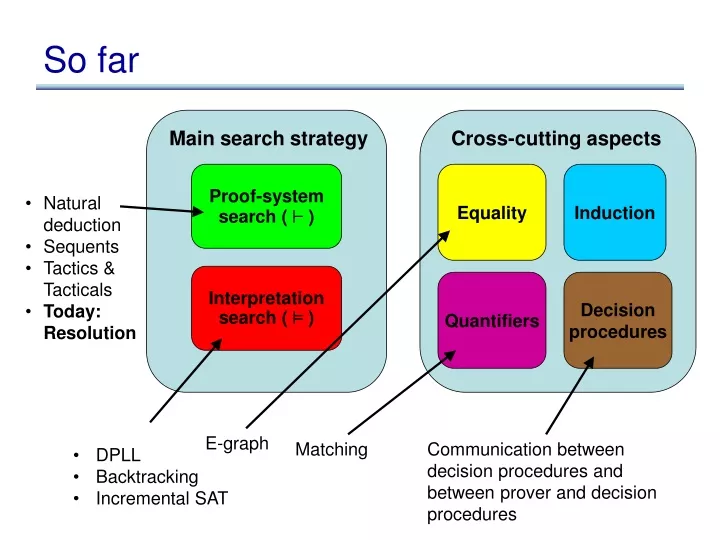
1. Main search strategy Cross-cutting aspects Proof-system search ( ` ) Equality Induction Interpretation search (² ) Quantifiers Decision procedures So far • Natural deduction • Sequents • Tactics & Tacticals • Today: Resolution E-graph Matching Communication between decision procedures and between prover and decision procedures • DPLL • Backtracking • Incremental SAT

2. Resolution • Originally developed by Robinson in 1965 • Most proof systems at the time had aimed at human reasoning. • They either: • Had many axioms (Hilbert style systems) • Or many inference rules (Natural deduction, Sequent calculus) • Robinson wanted to explore the possibility of having a simple calculus • with few but powerful axioms and inference rules • not necessarily intuitive form a human perspective, but more amenable to automated reasoning.

3. Resolution • Resolution calculus is far simpler than any of the other proof systems we have seen so far • There is only one axiom and one inference rule • This simplicity led many researchers to embrace the logic early on • One inference rule means that we can put all of our intellectual effort into making this rule efficient • Resolution is in fact still widely used today • Some of the most efficient fully automated theorem provers for first-order logic (E, Gandalf, Spass, Vampire) use variations of the resolution logic

4. Propositional resolution `)l  `l) RES `

5. Propositional resolution `)l  `l) RES `  ) 

6. Propositional resolution `)l  `l) RES `  )  `:Ç l  `:lÇ Expand ) RES ` :  Ç  `Ç l  `:lÇ Generalize RES `  Ç  `Ç lÇ  `Ç:lÇ RES Generalize even more `  Ç  Ç  Ç 

7. Propositional resolution `Ç lÇ  `Ç:lÇ RES `  Ç  Ç  Ç  resolvent

8. Propositional resolution Which direction should we apply this rule in? `Ç lÇ  `Ç:lÇ RES `  Ç  Ç  Ç  resolvent

9. Propositional resolution `Ç lÇ  `Ç:lÇ RES `  Ç  Ç  Ç  Assume , a, P`

10. Relation to other inference rules `Ç lÇ  `Ç:lÇ RES `  Ç  Ç  Ç 

11. Relation to other inference rules • Recall Modus Ponens: `Ç lÇ  `Ç:lÇ RES `  Ç  Ç  Ç  `l`l) MP ` `l`:lÇ  Expand ) MP ` MP is a special case of RES (with ,  and  set false)

12. Relation to other inference rules `Ç lÇ  `Ç:lÇ RES `  Ç  Ç  Ç 

13. Relation to other inference rules • Recall cut rule: `Ç lÇ  `Ç:lÇ RES `  Ç  Ç  Ç   ` , ll, ` CUT  ,  ` ,   ` , l` ,:l Throw l to the other side Resolution rule embodies the same idea as the cut rule from Sequents CUT  ,  ` ,  “Expand” definition of sequents  ` Çl` Ç:l  ,  ` Ç

14. `Ç lÇ  `Ç:lÇ Example Proof `  Ç  Ç  Ç  • Find a derivation of { : P Ç Q, S Ç P, : Q Ç R, : R } ` S

15. `Ç lÇ  `Ç:lÇ Example Proof `  Ç  Ç  Ç  • Find a derivation of { : P Ç Q, S Ç P, : Q Ç R, : R } ` S Is the proof unique?

16. `Ç lÇ  `Ç:lÇ Proof is not unique `  Ç  Ç  Ç  • Find a derivation of { : P Ç Q, S Ç P, : Q Ç R, : R } ` S

17. `Ç lÇ  `Ç:lÇ Another example `  Ç  Ç  Ç  • Find a derivation of: {} ` A Ç: A

18. `Ç lÇ  `Ç:lÇ Another example `  Ç  Ç  Ç  • Find a derivation of: {} ` A Ç: A • Can’t find a derivation • There are no clauses to resolve! • We made the calculus very simple (with only one axiom, and one inference rule) • but we also made it incomplete • What should we do?

19. Try refutation • We have seen refutation in the semantic domain • To show that a goal is valid, show that its negation is unsatisfiable • We can apply the idea in the proof domain • In the context of the proof domain: • To show that a goal is valid, assume its negation, and derive false

20. `Ç lÇ  `Ç:lÇ Try refutation `  Ç  Ç  Ç  • Find a derivation of: {} ` A Ç: A

21. `Ç lÇ  `Ç:lÇ Try refutation `  Ç  Ç  Ç  • Find a derivation of: {} ` A Ç: A • Refutation worked in this case • Q: Would it always work if the formula is valid?

22. Refutation • A: Yes • Although resolution is incomplete, it is refutation complete, which means that if the formula is valid, then adding its negation to the assumptions makes false provable • More formally… • Recall defn of completeness: • If ² then `

23. Refutation • A: Yes • Although resolution is incomplete, it is refutation complete, which means that if the formula is valid, then adding its negation to the assumptions makes false provable • More formally… • Recall defn of completeness: • If ² then ` • Defn of refutation complete: • If ² then , : ` false

24. Forward refutation-based resolution search • Keep a knowledge base, which is the set of formulas that have been inferred so far • Given goal to prove: • Add negation of goal to the knowledge base • While false not in knowledge base: • Choose two formulas to resolve • Add resolvant formula to the knowledge base • If false is in the knowledge base, return VALID • Is this search strategy complete?

25. Key issue: non-determinism • Source of non-determinism: need to determine which clauses to resolve • Two main approaches for handling these non-determinism • Simplification strategies • Ordering clauses

26. Simplification strategies • Simplification strategies remove redundant clauses from the knowledge base • Reduces number of choices, but also makes the search more space efficient • Example 1: remove a clause C if it contains a literal l that is not complementary with any other literal in the remaining clauses • Intuition?

27. Simplification strategies • Simplification strategies remove redundant clauses from the knowledge base • Reduces number of choices, but also makes the search more space efficient • Example 1: remove a clause C if it contains a literal l that is not complementary with any other literal in the remaining clauses • Intuition: l will never get resolved upon, and so resolvents derived from C (directly or indirectly) will therefore at least contain l, and thus cannot possibly be the empty clause

28. Simplification strategies • Example 2: tautologies can be removed, where a tautology can be detected by checking if a clause contains both a literal and its negation • Example 3: remove clauses that are implied by other clauses in the set • This is called subsumption • Various forms of it, depending on how the implication is tested, and when during the search the test is done

29. Ordering (clause selection) strategies • A good clause selection strategy is critical for finding proofs efficiently • Many ways to order clauses… • Just the E theorem prover (which won various automated theorem proving competitions) implements over 60 predefined clause selection schemes

30. Ordering (clause selection) strategies • Favor small clauses first, an instance of which is the idea of favoring one-literal clauses (unit resolution) • Favor old clauses • Corresponds to a FIFO order and leads to a breadth first ordering • Opposite strategy: always resolve the newest resolvent, which leads to a depth first search • Such strategies are called linear strategies because they create a linear chain of resolvents, each produced from the previous one • One such strategy, called SLD-resolution is at the core of Prolog

31. Example of SLD-resolution Assume: B1 B2 B1Æ B2) A (in prolog, written: A :- B1, B2 ) B3Æ B4) A (in prolog, written: A :- B3, B4) Query: A

32. Example of SLD-resolution Assume: B1 B2 B1Æ B2) A (in prolog, written: A :- B1, B2 ) B3Æ B4) A (in prolog, written: A :- B3, B4) Query: A

33. Another issue: finding complementary lits • Efficient data structures have been devised for efficiently finding complementary terms • Graph based data structure of Kowalski • Complementary literals connected with graph edges • When a resolvent is added, use existing edges in the graph to add the appropriate new edges • Indexing is another technique for efficiently determining which clauses to resolve • For example, answer queries such as: given a literal l, return all clauses that contain literals that unify with :l

34. First-order resolution • So far, we’ve seen propositional resolution • Now we’ll take look at the first-order case • However, before we do that, let’s take a detour to see a new technique for handling universal quantifiers in axioms: unification

35. Universals with unification • Given a universal axiom, our goal is to instantiate the universal with the right term t • Key idea • Instead of determining immediately what term to instantiate the universal, introduce a new fresh variable v which stands for the term t • At later stages in the proof, the variable v is gradually constrained until either its value is known, in which case the proof succeeds, or the system determines that no value for v is appropriate, in which case the proof fails • The constraints arise from unification

36. Overview of unification • Given two terms or formulas x and y, unifiy(x,y) returns a substitution  such that (x) is syntactically the same as (y). If no such  exists, the unification fails • Examples • unify(P(f(x),y), P(z, g(s)) = • unify(P(x,y), P(y,x)) = • unify(P(x, g(y)), P(f(y), x) = • unify(P(x), P(f(x)) =

37. Overview of unification • Given two terms or formulas x and y, unifiy(x,y) returns a substitution  such that (x) is syntactically the same as (y). If no such  exists, the unification fails • Examples • unify(P(f(x),y), P(z, g(s)) = • unify(P(x,y), P(y,x)) = • unify(P(x, g(y)), P(f(y), x) = • unify(P(x), P(f(x)) =

38. Example • Suppose we want to show: • 8 x . P(x) `8 x . P(f(x))

39. Example • Suppose we want to show: • 8 x . P(x) `8 x . P(f(x))

40. Careful! • Don’t confuse skolemization with the introduction of variables for later unification • Skolemization applies to universals that we are trying to prove, and it introduces constants • The introduction of fresh variables for unification applies to universals in assumptions, and it introduces variables • Although in some cases the difference between fresh variables and fresh constants is irrelevant, in the context of unification, the difference is important: • A variable can be unified with any constant, whereas a constant can only be unified with the exact same constant • For example, try showing f(0) `8 x . f(x)

41. Careful! • Don’t confuse skolemization with the introduction of variables for later unification • Skolemization applies to universals that we are trying to prove, and it introduces constants • The introduction of fresh variables for unification applies to universals in assumptions, and it introduces variables • Although in some cases the difference between fresh variables and fresh constants is irrelevant, in the context of unification, the difference is important: • A variable can be unified with any constant, whereas a constant can only be unified with the exact same constant • For example, try showing f(0) `8 x . f(x)

42. First-order resolution • We take the goal, negate it, and then: • We place the formula in prenex normal form, where quantifiers are on the outside • We remove existentials with skolemization (assumed existentials can be skolemized) • We are only left with universals, for which we introduce fresh variables, in the hope of doing unification later on

43. First-order resolution `Ç lÇ  `Ç:lÇ RES `  Ç  Ç  Ç 

44. First-order resolution `Ç lÇ  `Ç:lÇ RES `  Ç  Ç  Ç   = unify(l1 ,l2) `Ç l1Ç  `Ç:l2Ç Ç l1Ç and Ç:l2Ç have no common vars GEN-RES ` ( Ç  Ç  Ç )

45. Simple example • P(a,b) Ç: Q(a,b,c) , : P(s,t) Ç R(s)

46. Simple example • P(a,b) Ç: Q(a,b,c) , : P(s,t) Ç R(s)

47. Complete example 8 x. R(x, f(x,x)) ) 8 x. 9 y. R(x, y)

48. Complete example 8 x. R(x, f(x,x)) ) 8 x. 9 y. R(x, y)

49. Main search strategy review More human friendly, Less automatable Main search strategy • Natural deduction • Sequents • Resolution Proof-system search ( ` ) Interpretation search (² ) • DPLL • Backtracking • Incremental SAT Less human friendly, More automatable