Download
1 / 24
250 likes | 401 Views
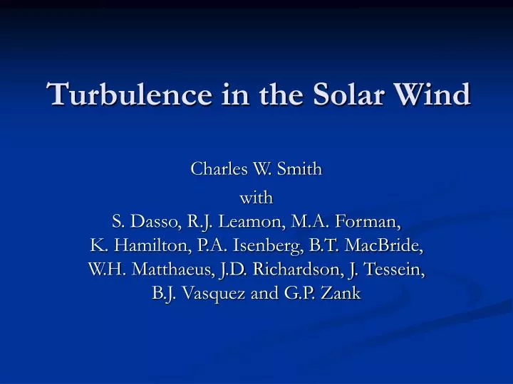
Turbulence in the Solar Wind. Charles W. Smith with S. Dasso, R.J. Leamon, M.A. Forman, K. Hamilton, P.A. Isenberg, B.T. MacBride, W.H. Matthaeus, J.D. Richardson, J. Tessein, B.J. Vasquez and G.P. Zank. Interplanetary Turbulence Spectrum. f -1 “energy containing range”. f -5/3

E N D
Turbulence in the Solar Wind Charles W. Smith withS. Dasso, R.J. Leamon, M.A. Forman, K. Hamilton, P.A. Isenberg, B.T. MacBride, W.H. Matthaeus, J.D. Richardson, J. Tessein, B.J. Vasquez and G.P. Zank
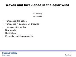
Interplanetary Turbulence Spectrum f -1“energy containing range” f -5/3 “inertial range” The inertial range is a pipeline for transporting magnetic energy from the large scales to the small scales where dissipation can occur. Magnetic Power f -3“dissipation range” Few hours 0.5 Hz
Why Turbulence? • Ultimate dynamics of the solar wind if left to its own devices. • Sets the rate of solar wind heating. • Partial responsibility for the manner of heating. • Controls the distribution of energy in spectrum. • Builds/destroys correlations responsible for charged particle scattering. • Dictates transverse magnetic fluctuations. • Directs wave vector away from field-alignment.
Observations of TP Approx. adiabatic prediction Solar Wind Heating In the range 0.3 < R < 1.0 AU, Helios observations demonstrate the following: For VSW < 300 km/s, T ~ R -1.3 0.13 300 < VSW < 400 km/s, T ~ R -1.2 0.09 400 < VSW < 500 km/s, T ~ R -1.0 0.10 500 < VSW < 600 km/s, T ~ R -0.8 0.10 600 < VSW < 700 km/s, T ~ R -0.8 0.09 700 < VSW < 800 km/s, T ~ R -0.8 0.17 We need to back out the heating rate as a point of comparison for inferred heating rates at 1 AU. This involves solving an equation like: Adiabatic expansion yields T ~ R-4/3. Low speed wind expands without in situ heating!? High speed wind is heated as it expands. Low-speed results have been corrected once in situ acceleration was considered.
~ u3/l Explaining the Heating Rate f -1“energy containing range” f -5/3 “inertial range” The inertial range is a pipeline for transporting magnetic energy from the large scales to the small scales where dissipation can occur. Magnetic Power f -3“dissipation range” Few hours 0.5 Hz
Non-adiabatic expansion Voyager 2 observations Turbulent heating model T / TS = (V / <V>) 3 – 2 with pickup ions bisphere Richardson & Smith, GRL, 30, 1206 (2003) full bisphere % bisphere Supply-Side Heating Theory • Z± = v ± b are Elsasser variables. • is the similarity scale = correlation length. T = proton temperature. • A = 1.1 • C = 1.8 • = 1 = Constrained by symmetry, Taylor-Karman local phenom., and solar wind conditions. Zhou and Matthaeus, JGR, 95, 10,291 (1990); Zank et al., JGR, 101, 17,093 (1996); Matthaeus et al., PRL, 82, 3444 (1999); Smith et al., JGR, 106, 8253 (2001); Smith et al., ApJ, 638, 508 (2006)
f -1“energy containing range” f -5/3 “inertial range” Magnetic Power The inertial range is a pipeline for transporting magnetic energy from the large scales to the small scales where dissipation can occur. f -3“dissipation range” Few hours 0.5 Hz Inertial Range Cascade
Energy Cascade Rate • The rate large-scale structures drive the turbulence • The rate of energy cascade through the inertial range. • The rate of energy dissipation in the dissipation range. • The rate of turbulent heating of the background plasma. • At 1 AU <> ~3 x 10³ Joules/kg-s
Inertial Range Characteristics • Strong correlation between V and B. • Signature of outward propagation. • Fluctuations perpendicular to the mean B0. • Large variance anisotropy (B/B > 1) • Signature of largely noncompressive fluctuations • Wave vectors both parallel and perpendicular to B0 • As shown by Matthaeus et al. and Dasso et al. • 5/3 power law index (Kolmogorov)
Milano et al., PRL, 93, 2004. Inertial Range Characteristics • Strong correlation between V and B. • Signature of outward propagation.
Smith et al., JGR, in press (2006) Inertial Range Characteristics NIMHD and WCMHD theories seem to imply a -scaling to the variance anisotropy. This represents balance between excitation and dissipation of compressive component. • Fluctuations perpendicular to the mean B0. • Large variance anisotropy (B2/B2 > 1) • Signature of largely noncompressive fluctuations
Slow wind is 2D Fast wind is 1D Matthaeus et al., JGR, 95, 20,673, 1990. Dasso et al., ApJ, 635, L181-184, 2005. Inertial Range Characteristics • Wave vectors parallel and perpendicular to B0 • As shown by Matthaeus et al. and Dasso et al.
To apply the Kolmogorov formula [Leamon et al. (1999)]: • Pk = CK2/3 k5/3 • Fit the measured spectrum to obtain “weight” for the result • Not all spectra are -5/3! I assume they are! • Use fit power at whatever frequency (I use ~10 mHz) • Convert P(f) → P(k) using VSW • Convert B2→V2 using VA via (V2 = B2/4) • Allow for unmeasured velocity spectrum (RA = ½) • Convert 1-D unidirectional spectrum into omnidirectional spectrum • = (2/VSW) [(1+RA) (5/3) PfB (VA/B0)2 / CK ]3/2 f5/2 f -1“energy containing range” f -5/3 “inertial range” Magnetic Power f -3“dissipation range” Few hours 0.5 Hz Leamon et al., J. Geophys. Res., 104, 22331 (1999) Inertial Range Characteristics • 5/3 power law index (Kolmogorov)
Beware! • Kolmogorov spectral prediction yields . • If the fluid is turbulent! • A static spectrum could yield a completely irrelevant prediction having nothing to do with anything. • Kolmogorov structure function prediction measures the strength of the nonlinear terms. • Only verification of an active turbulent cascade. • Politano and Pouquet (1998) extended structure function ideas to MHD. • We have recently applied these ideas to the solar wind at 1 AU. • See talk by Forman and poster by MacBride.
Power spectrum derivation of ~ 104 Joules/kg-s Energy and Dissipation Rates Cascade & dissipation rate is sufficient to dissipate the inertial range in 3-5 days and equilibrate outward and inward propagating waves. See Forman et al talk, this session.See MacBride et al. poster, this meeting.
f -1“energy containing range” f -5/3 “inertial range” Magnetic Power If the inertial range is a pipeline, the dissipation range consumes the energy at the end of the process. Ion Inertial Scale f -3“dissipation range” Inertial range spectrum ~ 5/3 Spectral steepening with dissipation Few hours 0.5 Hz The Dissipation Range
Hamilton et al., unpublished. Leamon Found: • Dissipation range spectrum highly variable. • Dissipation range has smaller variance anisotropy than inertial range. • Compressive component more important. • Quasi-perpendicular wave vectors are more aggressively damped than parallel vectors. • Cyclotron resonances is responsible for ½ 2/3 of energy dissipation.
Smith et al., ApJ, 645, L85, 2006. Transition to Dissipation • Traditional fluid turbulence requires: • Results from processes contained within the fluid approximation. • Onset of dissipation scales with ~ (3/)1/4. • Dissipation range spectrum is universal F(k). • The solar wind is not a traditional fluid! • Dissipation results from the breakdown of the single fluid theory. • At scales like (some number of) ion inertial scales.
Summary • Large-scale drivers of the turbulent cascade is able to account for the rate of heating the solar wind. • Issues with the rates determined from the inertial range. • Dissipation rate suggests that inertial range observations arise in situ. • Variance anisotropy scales with plasma . • Compressive component must be explainable via excitation/decay processes buried within turbulence. • Maybe maintaining association with initial conditions… • Onset of dissipation results from breakdown of fluid theory. • Cyclotron damping is only part of the story. • Most aggressive dissipation acts on the perpendicular wave vectors. • Dissipation range spectrum depends on the rate of cascade. • More compressive than inertial range. • More aggressive dissipation of k B0.
Leamon Found: • Dissipation range spectrum highly variable. • Dissipation range has smaller variance anisotropy than inertial range. • Compressive component more important. • Quasi-perpendicular wave vectors are more aggressively damped than parallel vectors. • Cyclotron resonances is responsible for ½ 2/3 of energy dissipation.
Non-Cyclotron Resonance Leamon et al., ApJ, 507, L181-184, 1998.