Download
1 / 27
270 likes | 383 Views
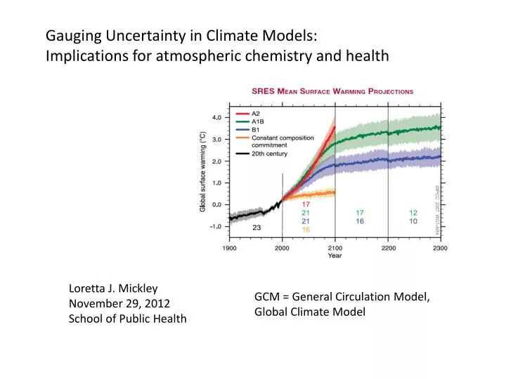
Gauging Uncertainty in Climate Models: Implications for atmospheric chemistry and health. Loretta J. Mickley November 29, 2012 School of Public Health. GCM = General Circulation Model, Global Climate Model. Basic working of climate models

E N D
Gauging Uncertainty in Climate Models: Implications for atmospheric chemistry and health Loretta J. Mickley November 29, 2012 School of Public Health GCM = General Circulation Model, Global Climate Model
Basic working of climate models All climate models depend on basic physics to describe motions and thermodynamics of the atmosphere: E.g., vertical structure of pressure is described by hydrostatic equation Climate models also depend on parameterizations for many processes. E.g., microphysics of cloud droplet formation, vegetation processes. Output Climate model Input Physics + Parameterized processes Tilt of earth, geography, greenhouse gas content Weather + Climate
Three ways to run a climate model. There are many variations! 1. Continually nudge model with observations from satellites, surface 1950 2000 2010 2050 2. Initialize with observed sea surface temperatures, then let run free. Force with observed greenhouse gas trends. 3. Run model forced by scenarios of greenhouse gases and aerosols. 4. Start centuries earlier with estimated ocean Ts. 5. Run with carbon cycle online.
particulate matter (PM) and ozone pollution emissions transport dilution chemistry population winds Winds carry pollutants to other boxes. Emissions + chemistry calculated within box Detour: how 3-D chemistry models work. GEOS-Chem chemical transport model: Global 3-D model describes the transport and chemical evolution of atmospheric pollutants Meteorology from a climate model
Validation of present-day climate models Temperature anomalies relative to 1901-1950 mean Observed global mean temperature anomalies 14 models, 58 simulations mean of models Models allowed to run freely, forced only by observed trends in greenhouse gases and aerosols. What causes spread in model response? IPCC, 2007
What causes spread in model response? • Climate chaos = “Butterfly effect” = noise, interannual variability • Starting the very same model with slightly different initial conditions will yield different day-by-day or year-by-year results. Temperature anomalies over eastern US Plot shows regional warming due to removal of US aerosol starting in 2010. Red dotted curves are results with same A1B forcing, but different initial conditions. Green is same but no US aerosol. Modelers run ensembles of simulations. 9-year running means Mickley et al., 2011
What causes spread in model response? 2. Differences in parameterizations or model resolutions, which lead to differences in model sensitivity to changing forcing. Global mean temperature response to 1% a-1 increase in CO2 for ~20 models. One simulation per model. Doubled CO2 IPCC, 2001
What causes spread in model response? 3. Unknown processes, lack of understanding of basic processes. E.g. aerosol indirect effect, aerosols provide cloud condensation nuclei. Range of estimates of aerosol indirect forcing in Wm-2 in present-day atmosphere varies greatly among many models. By comparison, CO2 forcing ~ +1.6 W m-2 IPCC 2007
The observed atmosphere also has “noise.” Temperature anomalies relative to 1901-1950 mean Observed global mean temperature anomalies Signal or noise? 14 models, 58 simulations mean of models IPCC, 2007 Even a “perfect” model cannot capture observed temperatures exactly because of climate chaos. Hard to tell what is signal and what is noise. How long should noise last? Years? Decades?
Another source of uncertainty in future simulations is the path of socio-economic development. Global mean surface temperature anomalies Different scenarios follow different socio-economic paths for developed and developing countries. A2 = heavy fossil fuel B1 = alternative fuels A1B = mix of fossil + alternative fuels IPCC 2007
Another source of uncertainty: abrupt climate change • Younger Dryas period= sudden cooling, followed by abrupt warming. • Greenland warmed by 7oC in a few decades. • Earth system hits a tipping point and is thrown into new state. • Possible triggers: • Loss of sea ice • Reversal in ocean currents Last Ice Age http://www.ncdc.noaa.gov
Future regional predictions for meteorology in A1B 2100 atmosphere show large variation across North America. Percent change in 2100 precipitation relative to present-day JJA Annual DJF Number of models showing increasing precipitation most models few models IPCC 2007
Exploring the uncertainty in climate models: big field of research Can we better characterize the spread of uncertainty in one model? Response of model to abrupt doubling of CO2 shows large spread. Global mean Temperature response to 2x CO2. Results from 90K simulations, each simulation with varied parameters for cloud processes. Large number of simulations needed to capture spread. Researchers colonized personal laptops across UK (like SETI project). Stainforth et al., 2005
Climate change and air quality • For the effect of climate change on air quality, we need to think about changes in episodic phenomena, e.g.: • Stagnation • Heat waves • Wildfires Probability of ozone exceedance • Reasons for increasing probability of ozone exceedances at higher max temps: • Greater stagnation + clear skies • Faster chemical reactions. • Greater biogenic emissions Northeast/ mid Atlantic in summer Probability maximum daily temperature (K) Lin et al., 2001
Calculation of maximum temperatures in climate models is sensitive to choice of parameters having to do with land cover/soil. Lower estimate Upper estimate Lower and upper estimates of JJA maximum temperatures in 2x CO2 atmosphere Central 80% range of increases for 44 versions of one climate model, with varying land cover parameters. oC 0 8 Forest roughness parameter Vegetation root depth Percent variability in Tmax accounted for by vegetation parameters. 6% 30% 50% Clark et al., 2010
Surface ozone levels are sensitive to cold-front passage. How will frequency of cold-front passages change in future? Leibensperger et al., 2008
Stagnation is also strongly correlated with high PM2.5. Correlations of PM2.5 with key meteorological variables. 1998-2008 meteorology + EPA-AQS observations Multiple linear regression coefficients for total PM2.5 on meteorological variables. Units: μg m-3 D-1 (p-value < 0.05) Increases in total PM2.5 on a stagnant day vs. a non-stagnant day. Mean PM2.5 is 2.6 μg m-3 greater on a stagnant day Tai et al. 2010
Dominant meteorological modes driving PM2.5 in much of Midwest and East are associated with cyclone passage. • Principal component (PC) decomposition of eight meteorological variables (xk)to identify dominant meteorological regimes that drive PM2.5 variability: Time series for dominant PC and deseasonalized PM2.5:Midwest in Jan 2006 2 PC 6 Observed PM2.5 (µg m-3) 1 3 PC 0 0 -1 -3 r = -0.54 -2 -6 PM2.5 • Dominant PC in Midwest consists of low T, low and rising surface pressure, strong NW wind. • Meteorology signals the arrival of a cold front. • Dominant PC in East is cyclone passage, in West is maritime inflow. Jan 28 Jan 30 Tai et al., 2011
Evaluation of present-day meteorological modes in AR4 climate models reveals differences among models. N42° W87.5° Observed 2 sample models Frequency (d-1) Modeled (2 IPCC models) and observed (NCEP/NCAR) 1981-2000 time series of frequency of dominant meteorological mode for PM2.5 in U.S. Midwest • Some models capture both the long-term mean and variability of meteorological mode frequency well. • As a first step, we use only those models that capture present-day mean and variability of frequency to predict future PM2.5
We compare the observed and AR4 modeled frequency of those meteorological modes driving PM2.5 variability across US. Modeled 20-year mean frequency (d-1) Observed 20-year mean frequency (d-1) Modeled (IPCC) and observed (NCEP/NCAR) 1981-2000 mean of frequency of dominant meteorological modes for PM2.5 in U.S. (western, central, eastern)
2000-2050 climate change leads to increases in annual mean PM2.5 across much of the Eastern US. We choose the 9 models whose frequency of the dominant meteorological modes best agrees with observations. We apply sensitivity of PM2.5 to changing frequency of dominant meteorological mode in the A1B atmosphere. Models show increased duration of stagnation, with corresponding increases in annual mean PM2.5. There is huge variation among models. day 1981-2065 change in period of dominant meteorological modes for PM2.5 variability averaged over 9 IPCC models mg m-3 Corresponding 1981-2065 change in annual mean PM2.5 concentrations (unit: µg m-3)
Another example: wildfires in the Western US in a future climate Our previous research has shown that area burned depends largely on temperature, precipitation, and relative humidity. Median change in key variables by 2050s relative to present-day, calculated by 14 AR4 models.
Models show large variation in changes in key wildfire variables across western US. Projected changes in key variables by 2050s, relative to present-day, across 6 ecoregions in the Western US. JJA only. PNW, Pacific Northwest CCS, California Coastal Shrub DSW, Desert Southwest NMS, Nevada Mountains /Semi-desert RMF, Rocky Mountains Forest ERM, Eastern Rocky Mountains /Great Plains.
Wildfire in Western United States in 2050s A1B climate. Ratio of 2050s area burned / present-day area burned Medians for all regions show increases in area burned. median Ratio of 2050s / present-day Eastern Rockies Nevada Mountains Pacific Northwest Rocky Mountatins Desert Southwest California Coastal Shrub
Given the uncertainties in climate models, how can atmospheric chemists/ epidemiologists proceed? • Compare signal of change to noise (interannual variability). • Look for those models that best capture present-day variables of relevance to atmospheric chemistry / health. Then use projections from only that subset of models. • Calculate the probabilities of specific changes. Most simply, give equal weight to all models/ensemble members, then calculate the percentage that show a specific effect.
Three ways to study chemistry-climate interactions. 2. Apply model chemical fields (ozone + aerosols) to climate model 1950 2000 2010 2050 3. Archive meteorology needed to run chemistry model. Climate model Physics + Parameterized processes +Chemistry 1. Implement chemistry scheme inside climate model! But this is computationally expensive. Chemistry can be simplified.