Download
1 / 39
470 likes | 933 Views
Quick Start Guide Leica SP5 X. Please note: Some of the information in this guide was taken from Leica Microsystems’ “ Leica TCS SP5 LAS AF Guide for New Users”. . Table of Contents. Page #. System Components Basic System Components………………………………..……...……………………………………………..1

E N D
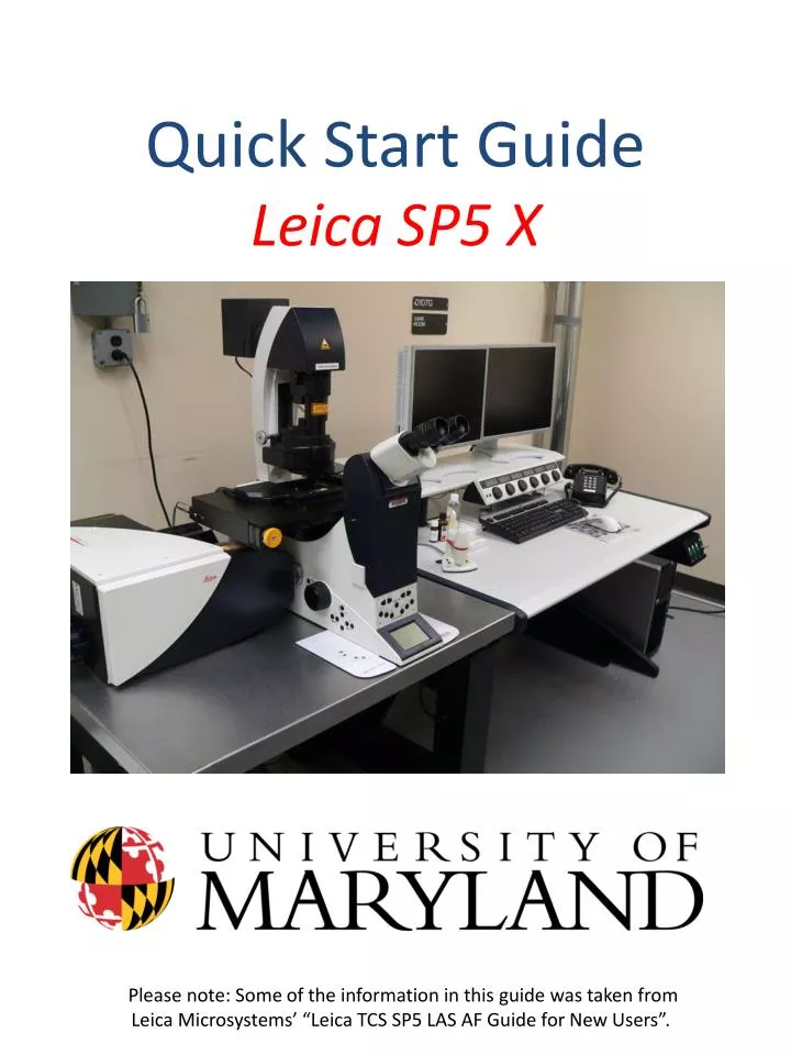
Quick Start GuideLeica SP5 X Please note: Some of the information in this guide was taken from Leica Microsystems’ “Leica TCS SP5 LAS AF Guide for New Users”.
Table of Contents Page # • System Components • Basic System Components………………………………..……...……………………………………………..1 • Basic Microscope Components…………………………………………………………….…………………..2 • System Start Up • Start the Hardware…………………..………………………………………………………………………………3 • Start the Software….……………….……………………………………………………………………………….4 • Find Your Sample • Choose an Objective Lens.………..…………...……………………………………………..…………………5 • Brightfield…………………………………………………………………………………………………………….….7 • Köhler Illumination…………………………………………..………………………………………….…………..8 • Fluorescence……..……………………………………………………………………………………………….……9 • Beam Path Settings • Configuration Window Overview………….………………………………………………………………..12 • Beam Path Settings………………………………..……………………………………………………………….13 • Beam Path Settings- Step by Step, DAPI Example……………………………………………….....16 • Sequential Scan Setup- FITC/TRITC example……………………………………….………………….17 • Scan the Sample • Visualize the Signal…..…………….…………………………………………………………………….……….24 • QLUT (“Range Indicator”) .……..…………………………………………………………….……………….25 • Modify the Image.……………………………………………………………………………….…………………26 • Improve Image Quality. .…………………………………………………………………………..……………28 • Z-Series • Setup……………………………………………………………………………………………………………………..29 • 3-D Projection • Maximum Intensity Projection………………………………………………………………………….……32 • 3-D Projection with Animation. ……………………………………………………………………….…….33 • Shutdown Procedure…………………………………………………….………………………………………34 • Appendix 1…………………………………………………….…………………………………..………………………35 • Appendix 2…………………………………………………….………………………………………………………..…36 • Appendix 3…………………………………………………….………………………………………………………..…37
System Components Heated Stage Power Supply Inverted Microscope Mercury Lamp Power Supply Scan Head Anti-Vibration table Stage controller White Light Laser Argon and 405 diode lasers
Microscope Components Condenser Lens Focus Knob Halogen Lamp Condenser Lens Mercury Lamp Power Supply Heated Stage Controller Stage controller Scan Head Focus Knob
Start the Hardware • Make sure the valve on the nitrogen tank is open. • If the valve isn’t open, contact the facility manager. • The pressure should read ~30 psi. If it doesn’t, contact the facility manager. • Turn on the mercury lamp power supply. • Sign the Log Sheet and record the number of hours displayed on the power supply counter in the ‘On’ space under ‘Time on Mercury Lamp’. • Turn on the ‘PC Microscope’ switch (#2), the ‘Scanner Power’ switch (#3) and the ‘Laser Power’ switch (#4). • The computer will start up automatically. Turn the Laser Safety key to the On-1 position. If using the white light laser, press the reset interlock button on the front of the laser (located to the left of the microscope).
Start the Software • Login to your Windows account. • Double click on the LAS AF icon to launch the software. • Check that the configuration is correct- “machine” should be selected if you are planning to scan new images. • If you need to use the resonant scanner, check the box “Active Resonant Scanner”. • Note- the Resonant Scanner is used for high speed imaging; ~ 29 frames/second @ 512x512 frame size, bidirectional scanning. It is very fast but results in a very noisy image.
Start the Software • When the window “Microscope Stand” pops up, select “No” unless you are planning to do advanced techniques such as image tiling or ‘’mark and find’. • Note! If you need to initialize the stage, you must first tilt the illumination arm (condenser arm) back away from the stage. Then click ‘Yes’. • Click on the ‘Configuration’ tab at the top and select ‘Laser’. • Activate the lasers you need by checking the appropriate boxes. • Note- if you are unsure which laser(s) to activate, check every box to make sure that the needed lasers will be turned on. If you’re using the Argon laser, make sure to put the digital power slider bar at 20-30%.
Find Your Sample: Choose an Objective Lens • Click on Acquire. • The window will automatically open to the Acquisition tab. • Click on ‘Objective’ in the main window and choose an objective lens from the drop down menu. • Available objective lenses: • 10x/0.4 NA Plan Apo Dry • 20x/0.7 NA Plan Apo Multi-immersion (water, glycerol or oil). • 40x/1.25 NA Plan Apo Oil • 40x/0.8 NA Water • 63x/1.4 NA Plan Apo Oil • 63x/1.3 NA Plan Apo Glycerine • Add the appropriate immersion media to your coverslip and place your slide coverslip side down over the objective lens. • If needed, use the x-y stage controller to move the stage so that your slide is positioned over the objective lens. • The top knob moves the stage in the y direction. • The bottom knob moves the stage in the x direction. • The buttons on the left side of the controller allow you to switch between fast and precise x-y movement. • Raise the objective lens up using the focus knobs until the lens just touches the immersion media on the coverslip. • Select Z Coarse or Z Fine on the stage controller and use the focus knobs on either side of the microscope or the z position knob (back knob) on the stage controller to focus. Z Y X
Find Your Sample: Brightfield • To find your sample using transmitted light, select the TL/IL button on the left side of the microscope. • The LCD screen on the front of the microscope should display TL_BF at the top. If it doesn’t, press the TL/IL button again. You can switch between brightfield and DIC by pressing the CHG TL button on the left side of the microscope. ‘CHG TL’ switches between BF, DIC and POL light ‘INT’ adjusts intensity of halogen or mercury lamp lamp Focus Knob ‘FD’ adjusts the mercury lamp field iris diaphragm ‘AP’ adjusts numerical aperture of condenser lens ‘TL/IL’ turns on transmitted light (halogen lamp; brightfield)
Find Your Sample: Köhler Illumination • Note- The confocal system can take transmitted (brightfield, DIC) images in addition to fluorescent confocal images. If you wish to take a transmitted light image of your sample, you should set up the microscope for Kohler illumination. If you are only taking fluorescent images of your sample, you do not need to perform Kohler illumination. • Set up the microscope for Kohler illumination. • Focus on your sample. • Close the field iris diaphragm. • While looking at your specimen through the eyepieces, focus the condenser until you see a small circle of illumination (this is the field iris diaphragm). Focus until the edges are clear and in sharp focus. 2 3
Find Your Sample: Köhler Illumination • Center the circle of light by turning the alignment pins. 4 • Open the field diaphragm back up so that you can see the entire field of view again. 5
Find Your Sample: Fluorescence • To find your sample using fluorescence microscopy, choose one of the filter sets on the front of the microscope and then press the SHUTTER button. • Available filter sets on the confocal system include: • GFP long pass filter, RFP, DAPI and CFP • When you’re finished looking at your sample, make sure to press the SHUTTER button again to avoid photobleaching your sample. • Note- You can adjust the intensity of the mercury lamp with the ‘INT’ button and the field diaphragm with the ‘FD’ button on the left side of the microscope. ‘INT’ adjusts intensity of halogen or mercury lamp lamp ‘FD’ adjusts the mercury lamp field iris diaphragm CFP DAPI
Image Acquisition Set Up • Click on Acquire. • The window will automatically open to the Acquisition tab. • The default scanning mode is xyz. • To change the mode, select another mode from the drop down menu. • The image format default is 512x512 pixels. • To change the imaging parameters, click on the arrowhead to open the dropdown window . • Note- Image size, as well as pixel size, is automatically calculated and displayed. Keep in mind that image format and the zoom factor affect pixels size, thus affecting image resolution. • To determine the correct pixel size for maximum resolution, see the Appendix 2. • The default speed is 400 Hz with a zoom factor of one. • Note- The fastest speed possible with a zoom factor of 1 is 600 Hz.. • At 700 Hz, the zoom factor increases to 1.7. • At 1000 Hz, the zoom factor increases to 3. • At 1400 Hz, the zoom factor increases to 6. • The default pinhole size is 1 Airy unit. • To change the pinhole size, check the box next to ‘Pinhole’ and adjust the settings. • Note- It is not recommended to decrease the pinhole size below 1 Airy unit. • Note- Increasing the pinhole size will increase your optical section thickness and allows more out of focus fluorescent light through to the light detector. • The default bit depth is 8. • For more information on bit depth, see Appendix 3.
Configuration Window Overview (Conventional lasers view) The tabs at the top allow you to switch between Conventional and White Light Laser views ‘Visible’ is the Argon laser- it has multiple lines ‘UV’ is the 405 diode laser You can choose a pre-configured single (simultaneous) setting from the drop-down menu To open a laser shutter, click on the radio button next to it- it will turn red when the shutter is open Laser power is adjusted using the slider bar Choose an objective lens here Spectral detection (emission) range is set and adjusted here There are 5 photomultiplier tubes (PMTs) for confocal imaging. Check the box under the PMT to activate it Transmitted light detector
Beam Path Settings • First, you’ll need to choose the appropriate laser(s) and laser line(s) to excite your fluorophore(s). • The SP5 X system is equipped with a 405 laser (‘UV), an argon laser (‘Visible’) and a white light laser (‘WLL’). • The choice of laser(s) will depend on the fluorophore(s) you are using • For example: FITC, GFP and Alexa 488 could all be excited by the 488 argon laser line or the 488 WLL laser line. Alexa 568 would be excited by the 568 line of the WLL and CY5 would be excited with the 633 WLL line. • To choose the 405 or argon laser, click on the button next to UV and/or Visible under the Conventional Lasers tab. • Select the laser and the intensity by moving the sliders up or down (start with no more than 20-30% power to begin with). • An active laser line will be expressed as a line on the spectrum.
Beam Path Settings • To choose a WLL excitation line, click on the White Light Laser tab. • Click on the radio button to open the WLL Shutter. • Select the desired wavelength by clicking on to drag the line or by clicking on the wavelength number and typing in a new wavelength. • Adjust the intensity by moving the sliders up or down (start with no more than 20-30% power to begin with). • An active laser line will be expressed as a line on the spectrum.
Beam Path Settings • To activate a PMT, click on the Active button and choose the color for your fluorophore emission. • A gray shadow will then appear underneath the PMT bar, confirming that the PMT is active. • Click on None to open the drop-down menu and choose the fluorophore emission wavelength. • This step will help you set your PMT spectral range. • Place the PMT bar in correspondence with the wavelength by sliding it left or right. • The slider can be resized by clicking to the right or left side of it and dragging. • The spectral range can also be chosen by double-clicking on the slider bar and typing in the spectral range. • Note- the spectral range minimum should always be set to at least 10nm greater than the excitation laser line. • For beam path setting examples, continue to page 16. For instructions on how to scan your sample, proceed to page 24.
Beam Path SettingsStep by step- Load single setting- DAPI example • There are several configurations already available in the software. • To choose a configuration, click on the fluorophore of choice from the Leica Settings drop-down menu in the ‘Load/Save single setting’ window. • Note- If you do not see your fluorophore listed, you can choose one that has an excitation/emission spectra similar to your dye and then modify some parameters (as discussed next). • As an example, let’s start with a setting for DAPI. When you click on DAPI, the software will: • Choose the appropriate laser for excitation • Open the laser shutter • Set an arbitrary laser power • Show the emission curve of the dye • Set an appropriate spectral range (emission range) • These settings can be modified…
Beam Path SettingsStep by step- Load single setting- DAPI example • Laser power • Laser power- can be increased or decreased by moving the digital slider arrow up or down OR by clicking on the laser power percentage and typing in a new number. The amount of laser power needed varies depending on the brightness of the sample. • Spectral detection window • To change the width or position of the spectral detector, double click on the slider bar and type in new minimum and maximum values or adjust the size of the slider bar by click on the arrows and dragging them to the left or right. • Note- A wide spectral range allows more light through to the detector. However, if the sample is labeled with more than one dye, a wide spectral range may increase the possibility of crosstalk (bleedthrough) between dyes. • Note, always set the minimum spectral range value at least 10nm higher than the excitation laser line. For example, when using the 405 laser, set the minimum range value no lower than 415nm. Setting the minimum value too close to the laser line will result in reflection of the laser into the light detector.
Beam Path SettingsStep by step- Load single setting- DAPI example • Image color • The color of your image can be changed by choosing a new color from the look-up table (LUT). If desired, click on the box next to the PMT and choose a new LUT from the available colors.
Beam Path SettingsSequential scan- FITC/TRITC example • In this section, we’ll set up a sequential scan for FITC (fluorescein) and TRITC (rhodamine) from scratch. • Note- sequential scanning will help reduce crosstalk/bleedthrough between dyes. However, keep in mind that scanning 2 channels sequentially will take twice as long as scanning them simultaneously. • Note- it is possible to load the FITC/TRITC single setting and then modify it to scan sequentially. To do this, click on Leica Settings in the Load/Save single setting box and click on FITC-TRITC. Continue on to step # to make this a sequential scan. • First, set up the FITC scan. • Choose the laser and excitation line. In this example, we’ll use the 488nm line of the white light laser (WLL), but it is also possible to use the 488nm line of the argon laser. • Make sure the WLL is on (See page 3 for information on how to turn on the lasers). • In the White Light Laser tab, open the laser shutter by clicking on the radio button next to ‘WLL Shutter’. The button will go from grey to red, indicating that the shutter is open. • Click on to drag one of the laser lines to 488nm and check the box to activate the line. You can also select the laser line by clicking on the wavelength and entering the desired wavelength number. • Increase the power by dragging the slider up. The number above the laser line indicates the percent power. Start with 10-20%.
Beam Path SettingsSequential scan- FITC/TRITC example • Set up the FITC scan (continued). • Activate PMT 2 by checking the ‘Active’ box below the PMT. • Load the FITC emission curve by clicking on ‘None’ and selecting FITC from the drop-down menu. • Double-click on the PMT 2 slider bar and type in the spectral range. Min= 505nm, Max = 550nm. • Click on the colored bar next to PMT 2 and choose the color green from the menu. The color selected here will be the color of your scanned image.
Beam Path SettingsSequential scan- FITC/TRITC example • Add the TRITC (rhodamine) scan. • In the White Light Laser tab, make sure the laser shutter is open (the radio button next to ‘WLL Shutter’ should be red). • Click on to drag one of the laser lines to 552nm and check the box to activate the line. You can also select the laser line by clicking on the wavelength and entering the desired wavelength number. • Increase the power by dragging the slider up. The number above the laser line indicates the percent power. Start with 10-20%. • Activate PMT 3 by checking the ‘Active’ box below the PMT. • Load the TRITC emission curve by clicking on ‘None’ and selecting TRITC from the drop-down menu. • Double-click on the PMT 3 slider bar and type in the spectral range. Min= 565nm, Max = 700nm. • Click on the colored bar next to PMT 3 and choose the color red from the menu. The color selected here will be the color of your scanned image.
Beam Path SettingsSequential scan- FITC/TRITC example • So far, we’ve set up a simultaneous scan for FITC/TRITC. Now we need to set it up as a sequential scan. • Click on Seq. in the Acquisition Mode menu. • In the Sequential Scan window, select the radio button • next to ‘between lines’. This means the software • will scan sequentially line by line. It is also possible • to scan sequentially frame by frame. • Click on the (+) button to add an additional scan. • Highlight Scan 1 by clicking on it once. • Now we’ll set up Scan 1 to scan FITC only. To do • this, uncheck the box under the 552nm laser line • to deactivate the 552nm line of the laser. • Deactivate PMT 3 by unchecking the ’Active’ box • under PMT3.
Beam Path SettingsSequential scan- FITC/TRITC example • FITC/TRITC sequential scan setup continued… • In the Sequential Scan window, highlight Scan 2 by clicking on it once. • Now we’ll set up Scan 2 to scan TRITC only. To do • this, uncheck the box under the 488nm laser line • to deactivate the 488nm line of the laser. • Deactivate PMT 2 by unchecking the ’Active’ box below PMT 2. • The Sequential scan is now set up. First, the 488nm laser line will scan one single line of the sample and the emission (FITC) will be collected using PMT2. Next, the 552nm line will scan and the emission (TRITC) will be collected in PMT3. This process will be repeated, with each laser and PMT being activated one after another, line after line, until the whole image has been scanned. For example, if the image format is set to 512 x 512, the process will be repeated 512 times.
Scan the SampleVisualize the signal • Make sure you have chosen the correct beam path settings and check to make sure your scan parameters are set up correctly. • If this is your first time scanning, I suggest keeping the default values (512x512 format, 400Hz, Zoom 1. See page *** for more details. • Click on the Live button (lower left corner of the setup screen) to check a live image of your sample. • Turn the Smart Gain knob until you can visualize the signal. If you have 2 PMTs activated, then your screen will be separated into 2 halves. • Click on one half of the viewing screen to select the channel, then adjust your gain using the Smart Gain knob until you can visualize the signal. The gain is the voltage on your PMT; it ranges from 0-1250 volts. Increasing the gain will increase the sensitivity of your PMT. • Click on the other half of the screen to select the other channel and adjust the gain for this channel using the Smart Gain knob again. Increase the Smart Gain until you see a signal Click on one half of the viewing screen to select the channel
Scan the SampleQLUT • Click on the QLUT (Quick Look Up Table) to show pixel intensity values in your image. • Note- the default bit depth of the image is 8, meaning your image will contain 256 gray levels. Each each pixel in your image will be scaled between 0 (black) and 255 (white). For more information on bit depth, see Appendix 2. • Your image will now be displayed in a glow scale mode. • The deeper shades of orange in the image indicate lower intensity values, lighter orange values indicate mid-range intensity pixels and white pixels are the brightest. • The color blue indicates a pixel is saturated (value of 255 or greater). • Background pixels, having an intensity of 0 or below, are colored in green. Blue= saturated Signal= 255 or > Gain adjustment Black to Orange to white= Signal between 1 to 254 Green = no signal = 0 or below Offset adjustment 255 8-bit image= 256 shades of grey Useful pixels: Signal from 1 to 254 0
Scan the SampleModify the Image • Adjust the Smart Gain and Offset to change the intensity values in your image. • Use the Smart Gain to reduce pixel intensity values until there are very few blue pixels in the image. Keep in mind any pixel colored blue is saturated, meaning it has an intensity value of 255 or greater. These pixels cannot be quantified. • Use the Smart Offset to adjust the image background until there are a few green pixels in the background of the image. • Note- the default Smart Offset value is very sensitive and makes it difficult to adjust your background. To change the sensitivity of the dial, click on Control Panel in the configuration window, select the Smart Offset button on the screen and change the sensitivity to 1 or 0.1% per turn. • Your final image should have a few blue pixels (unless you need to quantify those pixels- in that case you should have no blue pixels), mostly orange and white pixels, and a few green pixels in the background. Blue= saturated Signal= 255 or > Gain adjustment Black to Orange to white= Signal between 1 to 254 Green = no signal = 0 or below Offset adjustment
Scan the SampleModify the Image • Adjust laser intensities if necessary. • If the image is still too dim or not visible at all, enhance the laser power using the vertical slider until you can see an image on the screen. • Note- if the Smart Gain is lower the ~500 V, try decreasing the laser power and increasing the gain until about 900-1000 V. This will help reduce photobleaching of the sample. • Note- if the Smart Gain value is greater than ~1100 V, try increasing the laser power and lowering the Smart Gain. This will help reduce noise in the image. • Because higher laser power can cause increased photobleaching, it is best to try and keep laser power as low as possible. • Adjust the spectral detection window(s) if necessary. • Ensure the spectral window is positioned to include the emission maxima of your dye, as shown in the example below. • The window can be adjusted from side to side or expanded. Always make sure the minimum value is at least 10nm greater than the excitation laser line. In this example, the minimum value would be 498nm. • When you’ve finished adjusting the image, click on the stop button and then click on the Capture Image button to acquire an image.
Scan the SampleImprove Image Quality • There are several steps you can take to improve the quality of your image. • Rather than taking one single image of your sample, try averaging lines or frames. • For example, a Line Average of 2 means that each line of your sample will be scanned twice and the average of the two images will be displayed. • Frame Averaging works in a similar manner, except the whole frame is first scanned once and then scanned a second time. The final image is the average of both scans. • Taking an image using Line or Frame averaging will slow down the speed of image acquisition. For example, an Line Average of 2 will take twice as long to scan as a single image (Line Average 1). • Line and Frame Averaging will also increase photobleaching. • Try slowing down the scan speed. • Scanning more slowly can improve the quality of your image. • Keep in mind that it will take longer to scan your image. • Scanning more slowly will also increase photobleaching. • In general, lower Gain values will result in an improved image. • In order to use lower Gain, laser power must be increased. • Be careful when using higher laser power as this can photobleach or even damage your sample. • Make sure you are using the appropriate objective lens, Image Format and Zoom level. • Higher numerical aperture lenses will produce higher resolution images. • Increasing the Image Format size will also increase image resolution. • See Appendix 2 (page ) for additional information on how the objective lens, Image Format and Zoom level effect your image. • Adjust the pinhole size if necessary. • A pinhole size of 1 Airy Unit will result in the best possible resolution in the z-axis. • However, in cases where the signal is very low, opening up the pinhole will allow more light through to the detector and can result in a better looking image in the x-y plane. • Keep in mind that opening the pinhole means more out of focus fluorescent light is allowed to pass through to the detector, reducing resolution in the Z-axis.
Z-Stack • Make sure you are in xyz Acquisition Mode. • Click on the Z-Stack window. • Choose either z-Galvoorz-Wide. • In the z-Galvo method, the objective lens turret is held stationary and the stage (z-galvo stage) is moved up and/or down to change the focus position The maximum travel range is 500um. The z-Galvo stage can change focal positions more quickly than the z-Wide method and is recommended for high-speed z-series image acquisition. • In the z-Wide method, the stage is held stationary and the objective lens nosepiece is moved up and down to focus. The maximum travel range is 9000um. • Click on the Live button to start scanning. • Using the Z-position knob, move to the top of the sample (or region of interest). • Turning the knob in the counter-clockwise position moves the focal position closer to the coverslip (top of your sample). • Click on the Begin arrowhead (the arrowhead will go from black to brick-colored). • Using the Z-position knob, move to the bottom of your sample (or region of interest). • Turn the knob clockwise to focus deeper into the sample (away from the coverslip). • Click on the End Arrowhead.
Z-Stack • Click on Stop. • To set the number of z-steps, choose ‘System Optimized’ if you desire to obtain the optimal number of images calculated for your z-stack size (depending on the objective lens, zoom and image format). • If your goal is to create 3-D images from your Z-stack data, it is best to leave the system optimized or close to optimized. Keeping the system optimized ensure correct (Nyquist) sampling and will ensure you are not missing any image information between slices. • If you choose to change the number of steps, click on Nr. of steps or Z-step size and then enter a new value. • Click on Start and your Z-stack will begin and end automatically.
3-D ProjectionMaximum Intensity Projection • After acquiring a z-stack, it is possible to make a maximum intensity projection. • Under the Experiments tab, select the Series name. • Go to Process. • Click on Tools. • In the Process Tools, click under Visualization and 3D Projection, located at the bottom of the list. • Do not change the X,Y and Z planes if you just need a simple projection. • Enter Maximum in the Method drop down list (Average can be used if your fluorescence intensity is very strong and a maximum intensity projection completely saturates the signal). • Enter 1 in the Slice Thickness. • Click on Apply. 2 3 4 5 7 8 9
3-D Projection3-D Animation • After acquiring a z-stack, it is possible to make a 3-D Animation. • Under the Experiments tab, select the Series name. • Go to Process. • Click on Tools. • In the Process Tools, click under Visualization and 3D Projection, located at the bottom of the list. • Click on Create Movie. • Enter the Start Rotation angel (in degrees). For example, -45 degrees in Y. Click on Set Start. • Enter the End Rotation angle (in degrees). For example, +45 degrees and click on Set End. • Under options, enter the Method in the drop down list (for example: Maximum). • Enter the Number of Frames (the higher the number and slower the speed of rotation; for example: 70 for a complete rotation for a 512 x 512 z-stack series. • Click on Apply. 2 3 4 5 9 10 7 8 6 11
Shutdown Procedure • Check the microscope schedule. If someone is scheduled to use the microscope within an hour, simply close the software, log out of your Windows account, clean the objective lenses you used and fill out the log sheet. • If no one is scheduled to use the microscope for more than an hour after you are finished with the microscope, shut down the microscope completely, as detailed below: • Save your images. • In the laser configuration tab, uncheck all the lasers. • Exit the software. • Log out of your Windows account and shutdown the computer. • Clean the objective lenses you used with Sparkle and lens paper. • Press the Z button on the right side of the microscope to lower the objective lenses down. • Turn the laser safety key to the “Off-0” position. • If you used the argon laser, wait approximately 2 minutes for the argon cooling fan to click off before proceeding with the shut down. • Turn off Laser Power (#4), then Scanner Power (#3), then PC Microscope (#2). Uncheck
Shutdown Procedure • Fill out the log book. Record the time from the mercury lamp power supply in the “OFF” space of the user log. Indicate which objective lenses you used and how you left the microscope. • Turn off the mercury lamp. • Put the cover on the microscope!
Appendix 1: Lasers • Argon Laser • Allow approximately 15 minutes for the laser to warm up fully before performing quantitative or critical imaging experiments. • The Argon laser has lines at 458, 476, 488, 496 and 514nm. • For routine imaging, make sure to move the digital slider bar to 20-30% output. • For certain applications where very high laser power is needed (such as FRAP), the laser output can be increased. • The Argon laser power is distributed unevenly. • 458nmline: 5mW • 476nm line: 5mW • 488nm line: 20mW • 496nm line: 20mW • 514nm line: 20mW • Examples of dyes that can be used with the argon laser include: CFP (458nm), GFP and FITC (488nm) and YFP (514nm). • 405 diode laser • Does not require any warm up time before imaging. • 50mW laser. • Suitable for DAPI, Hoescht and photoactivation. • White Light Laser (WLL) • Allow approximately 1 hour for the laser to warm up fully performing quantitative or critical imaging experiments. • The WLL is tunable in 1nm increments between 470-670nm. • Up to 8 lines (8nm apart) can be used simultaneously. • Each line of the WLL averages 1.5mW. The shorter wavelengths typically have slightly less power than the longer wavelengths.
Appendix 2- Image format, zoom, pixel size and resolution… • Follow these steps to collect a high resolution image. • Choose your objective lens. • First, consider what you are trying to image. What is the smallest structure you will need to resolve? Use this information to choose an objective lens. Remember, objective lenses with higher Numerical Apertures (NA) will have greater light gathering ability and greater resolving power. • The highest NA lens on our system is the 63x/ 1.4 NA oil lens on our system. • Start with a 512 x 512 image format. • Formats range from 16 x 16 up to 8k x 8k • The image format indicates the number of pixels in your image. For example, a 512 x 512 format size means your image is composed of 512 pixels in both the x and y direction (a total of 262,144 pixels). • Choose the correct zoom power. • Monitor the pixel size as you zoom in. • The table to the right shows the target pixel size of each lens. For example, the target pixel size for the 63x oil lens is 91nm. If the pixel size is greater than 91nm, you are not taking full advantage of the resolving power of the 63x lens. Pixels sizes below 91nm results in oversampling. • Keep in mind that increasing the zoom factor increases photobleaching • Increase the image format if needed. • If the pixel size is still to large to resolve the structure you are trying to image or if you require a larger field of view, increase the format size. Keep in mind that an increase in format size results in a much bigger file size. Note- for additional information on this topic, see LeicaConfocal Application Notes, Vol. 3: “On Resolution, Pixels, Zoom and Scan Format”
x y Appendix 3- Bit Depth Explained • When your sample is scanned, the emitted fluorescence signal is detected by a PMT (photomultiplier) and converted into digital picture elements (pixels). • Each of these pixels has a specific intensity value. The range of intensity values you collect depends on the bit depth you select. • 8 bit data depth will give 256 gray levels - each pixel in your image will be scaled between 0 (black) and 255 (white). • 12 bit data depth will result in 4096 gray levels. • 16 bit data depth results in 65535 gray levels. • To change the bit depth, click on Configuration, Settings, and select 12 or 16.