Download
1 / 31
310 likes | 472 Views
From Telegraph Double Dotting To Microwave QPRS (Quadrature Partial Response Signalling). George de Witte VE3AYB QCWA Sep 20, 2011. Background 19 th Century Telegraphy. 1837 Wheatstone 5 needle, 6 wire system Euston-Camden Town 1852 6000 miles of 6 wire Telegraph in UK

E N D
From Telegraph Double Dotting To Microwave QPRS (Quadrature Partial Response Signalling) George de Witte VE3AYB QCWA Sep 20, 2011
Background 19th Century Telegraphy • 1837 Wheatstone 5 needle, 6 wire system Euston-Camden Town • 1852 6000 miles of 6 wire Telegraph in UK • 1850 Dover-Calais Single Wire Cable based on Gutta-Perra insulator • Soon after many other short distance submarine cables in Europe • 1858 First Transatlantic Cable from Ireland to NewFoundland • It worked for 3 days, it took hours to send a few words • Unknowns : cable strength, armour, dispersion, HV breakdown • Cable laying and Cable recovery • 1866 Second Transatlantic Cable • Recent submarine survey found “plateau” in North Atlantic • Stronger Cable 1 inch, but weighed 9000 tonnes/ 2300 miles • Was more successful and inspired many more cables
The Economic Reality • The investments were high >1M$ in 1865 $$’s • A cable laying ship had 2000 men on board (and livestock to feed them) • A skilled Telegraph Operator was paid as much as a Bank Manager • Operating Speed was 8 WPM • Telegram Tariff for 20 words incl address was $150 • Despite all that 21 transatlantic cables by 1928 The incentive to improve speed was phenomenal
Key Theoretical Contribution by Lord Kelvin • The common belief was that higher battery voltage was required • The first 1858 cable was likely destroyed by High Voltage • In 1855 he contended that the cable speed was proportional to the square root of the length • He defined what we today call pulse dispersion R R R R C C C
Cable Laying Ship The Great Eastern Cable ship measured ship-shore continuity during laying
Shore end Cross-section Shore end of Cable Stripped Deep Sea Cross-section
Nyquist Theory 1928 Channel Response Transmit Filter Receive Filter Output Data Input Data Noise Sampler & Threshold Detector C(f) Gt(f) Gr(f) + Xn Xn X(f) BPF BW=Fnyquist LPF BW=0.5Fnyquist X(f)=Gt(f)*C(f)*Gr(f) X(f)=T ) X(f)=0 ) -1/2T<f<1/2T sin πt/T x(t)= ------------- πt/T F=1/T is called Nyquist frequency 0
More Nyquist Theory ( T 0<f<(1-α)/2T X(f)= ( (T/2[1-sin(πT(f-1/2T)/α)] (1-α)/2T <f<(1+α)/2T sin πt/T cos απt/T x(t)= ------------- ---------------- πt/T 1-4α2t2/T2 - 6 dB point 1/2T 1/T
Eye Pattern 30% Raised Cosine • In a perfect Raised Cosine Channel the Intersymbol Interference is theoretically zero • Cable Attenuation is well known to be proportional to sqrt(f*L) • The sqrt(f) response approximates a raised cosine response with large α • Therefore the max cable speed is at the 6 dB down cable attenuation ie the Nyquist frequency
Duobinary Concept • Doubles the speed • First mentioned by A Lender in 1963 paper. • Also called Partial Response • Easiest implementation is a simple digital filter 1011 1V,-1V 2V,0,-2V Xn Binary To Bipolar + + 3 Level Encoder Out Nyquist Filter Σ Data In + 1 symbol delay T Xn-1 Data In 1 0 1 1 1 0 0 0 1 0 1 0 Bipolar Data In 1 1 -1 1 1 1 -1 -1 -1 1 -1 1 -1 + Xn + Xn-1 (3 Level) 2 0 0 2 2 0 -2 -2 0 0 0 0
Duobinary Decoder 1011 1V,-1V 1011 2V,0,-2V 1V,-1V Binary To Bipolar + Slicer And Sampler Bipolar to Binary + Nyquist Filter Σ Σ - + 1 symbol delay T 1 symbol delay T Data Out Data In Data In 1 0 1 1 1 0 0 0 1 0 1 0 Bipolar Data In 1 1 -1 1 1 1 -1 -1 -1 1 -1 1 -1 Xn + Xn-1 (3 Level) 2 0 0 2 2 0 -2 -2 0 0 0 0 - Bipolar Data Out 1 -1 1 1 1 -1 -1 -1 1 -1 1 -1 Data Out 1 0 1 1 1 0 0 0 1 0 1 0
Some More Duobinary Theory + Encoder is a Digital Filter H(f)=1+e-j2πfT Euler’s Formula : H(f)=cos (πfT) Σ Xn + Xn-1 1 symbol delay T - 6 dB point 1 H(f)=cos (πfT) 0.5 1/2T 1/3T f -2T -T 0 T 2T 3T
Eye Pattern Duobinary • Duobinary can also be achieved with a cosine shaped Low Pass Filter • With a perfectly truncated cosine frequency response the Intersymbol Interference is zero. • The 6 dB down frequency is 0.6 * raised cosine case • For the same cable attenuation, the signalling speed for duobinary is almost double the binary raised cosine case
Double -dotting • In 1898 Gulstad published paper : “Vibrating Cable Relay” • In hindsight invented Duobinary long before Lender in 1963 • Up until then cables were run at the “natural” speed (ie Nyquist Frequency) • He proposed doubling the speed, so that a 10101 dotting pattern resulted in almost zero Voltage output on the cable • As decoder on the Receive side he used a Polarized Relay with 2 extra windings • Each extra winding was connected with its own battery and RC network • The battery voltage and RC values were carefully adjusted so that one winding cancelled the second half of a detected + pulse and the second extra winding did the same for a –pulse • Gulstad called it “Vibrating Cable Relay” because in the absence of a cable signal, it vibrates at the “natural” frequency
Long Haul Microwave • In US Bell Labs centre of expertise compliments DoD • Radar technology during WWII advanced microwave technology • Post war economic boom demanded intercity TV and telephone • First microwave was TD-2 • All vacuum tube, key part 416C planar microwave tube • Operated in 4 GHz band, 240 Voice channels or 1 TV • 1950 First Route NYC- Chicago • 1958 First Canadian coast to coast route
Microwave status mid 70’s • Equipment all solid state except TWT amplifier (10 watt) • Telephone companies “owned” 4 GHz common carrier band • 12 RF duplex channels 20 MHz each • Separate Transmit/Receive antenna’s • Easy to recognize Bell Type A towers with 2+2 horn reflector antenna's • Capacity 1 TV or 1200 VF channels • Modulation FDM-FM (FDM=SSB-SC with 4 KHz spacing) • Everybody else (CN-CP, Western Union, MCI) “owned” 6 GHz band • 8 RF duplex channels 30 MHz each • Duplex 10-12 ft parabolic antenna’s • Capacity 1 TV or 1800 VF Channels
Digital World was coming in 1976 • Bell Northern Research was working on DMS digital CO switch • The “toll” interface was digital • Technology existed for intra-city digital transmission • T1 carrier @ 1.544 Mb/s • Hence a need developed for intercity digital microwave
Requirements for a Digital Microwave • Overbuild on existing 4 GHz network • CRTC made 8 GHz band available in Canada • Channel plan was 40 MHz • VF capacity similar to existing analog FDM-FM ie 1200+ • Digital Hierarchy DS-1 1.544 Mb/s 24VF • DS-2 6.312 Mb/s 96VF • DS-3 44.736 Mb/s 672 VF • By default capacity was set at 2 DS-3 (1344VF) or 91 Mb/s • Modulation efficiency requirement 2.25 bit/sec • FCC/CRTC defined a spectral emission mask (Spectrum Management)
Choice of Modulation Method • Constraint; cost of TWT amplifier • Amplitude and phase nonlinearity of TWT • Modulation candidates • 8PSK very difficult to implement, but constant envelope • 16QAM 4 level PAM on I and Q axis AM vs TWT • QPRS 2 level QAM on I and Q axis => TWT => filter => QPRS • Filter can be split between Transmitter and Receiver • Transmit Filter standard Tchebyshew and meets FCC Q-axis 4QAM QPRS I-axis 4QAM Rcvr Filter Trmt Filter TWT Baseband μW
QPRS Eye Pattern Q-axis I-axis
Transmitter Implementation Data 90 Mb/s Data 45 Mb/s 2L 70MHz I-signal 2 Level AM Modulator 4QAM 8 GHz 0 deg 4QAM 70 MHz Σ Up- converter 0/90 deg Phase Splitter Serial To Parallel TWT Amp ½QPRS BPF 90 deg 2 Level AM Modulator 2L 70MHz Q-signal 8 GHz Oscillator 70 MHz Oscillator
Receiver Implementation 3 Level I-signal 45 Mb/s I data + Σ ½QPRS LPF 2 Level AM Demod Data Detector 90 Mb/s - 0 deg 1 Symbol delay Down Converter 70 MHz AGC Amp 0/90 deg Phase Splitter Parallel To Serial 3 Level Q-signal 90 deg + Σ 2 Level AM Demod ½QPRS LPF Data Detector - 1 Symbol delay 8 GHz Oscillator 70 MHz Carrier Recovery 45Mb/s Q Data
Summary • Field Trial held 1976 Avonmore –Kemptville • Impact of Propagation much worse than expected • Added Space diversity with Phase-Adaptive Combiner at 70 MHz • Added Automatic Amplitude Slope Equalizer • Commercial Introduction 1978 Toronto-Winnipeg • Eventually Extended coast-to-coast • The Worlds First successful Long Haul Digital Microwave