Download
1 / 58
580 likes | 966 Views
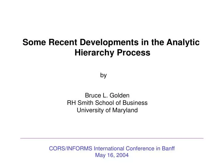
Some Recent Developments in the Analytic Hierarchy Process. by. Bruce L. Golden RH Smith School of Business University of Maryland. CORS/INFORMS International Conference in Banff May 16, 2004. Focus of Presentation. Celebrating nearly 30 years of AHP-based decision making AHP overview

E N D
Some Recent Developments in the Analytic Hierarchy Process by Bruce L. Golden RH Smith School of Business University of Maryland CORS/INFORMS International Conference in Banff May 16, 2004
Focus of Presentation • Celebrating nearly 30 years of AHP-based decision making • AHP overview • Linear programming models for AHP • Computational experiments • Conclusions 1
AHP Articles in Press at EJOR • Solving multiattribute design problems with the analytic hierarchy process and conjoint analysis: An empirical comparison • Understanding local ignorance and non-specificity within the DS/AHP method of multi-criteria decision making • Phased multicriteria preference finding • Interval priorities in AHP by interval regression analysis • A fuzzy approach to deriving priorities from interval pairwise comparison judgments • Representing the strengths and directions of pairwise comparisons 3
A Recent Special Issue on AHP • Journal: Computers & Operations Research (2003) • Guest Editors: B. Golden and E. Wasil • Articles • Celebrating 25 years of AHP-based decision making • Decision counseling for men considering prostate cancer screening • Visualizing group decisions in the analytic hierarchy process • Using the analytic hierarchy process as a clinical engineering tool to facilitate an iterative, multidisciplinary, microeconomic health technology assessment • An approach for analyzing foreign direct investment projects with application to China’s Tumen River Area development • On teaching the analytic hierarchy process 4
A Recent Book on AHP • Title: Strategic Decision Making: Applying the Analytic Hierarchy Process (Springer, 2004) • Authors: N. Bhushan and K. Rai • Contents Part I. Strategic Decision-Making and the AHP 1. Strategic Decision Making 2. The Analytic Hierarchy Process Part II. Strategic Decision-Making in Business 3. Aligning Strategic Initiatives with Enterprise Vision 4. Evaluating Technology Proliferation at Global Level 5. Evaluating Enterprise-wide Wireless Adoption Strategies 6. Software Vendor Evaluation and Package Selection 7. Estimating the Software Application Development Effort at the Proposal Stage 5
Book Contents -- continued Part III. Strategic Decision-Making in Defense and Governance 8. Prioritizing National Security Requirements 9. Managing Crisis and Disorder 10. Weapon Systems Acquisition for Defense Forces 11. Evaluating the Revolution in Military Affairs (RMA) Index of Armed Forces 12. Transition to Nuclear War 6
AHP and Related Software • Expert Choice (Forman) • Criterium DecisionPlus (Hearne Scientific Software) • HIPRE 3+ (Systems Analysis Laboratory, Helsinki) • Web-HIPRE • Super Decisions (Saaty) EC Resource Aligner combines optimization with AHP to select the optimal combination of alternatives or projects subject to a budgetary constraint The first web-based multiattribute decision analysis tool This software implements the analytic network process (decision making with dependence and feedback) 7
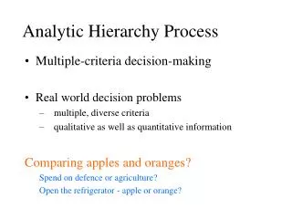
AHP Overview • Analysis tool that provides insight into complex problems by incorporating qualitative and quantitative decision criteria • Hundreds of published applications in numerous different areas • Combined with traditional OR techniques to form powerful “hybrid” decision support tools • Four step process 8
The Analytic Hierarchy Process • Step 1. Decompose the problem into a hierarchy of interrelated • decision criteria and alternatives Objective Level 1 … Criterion 1 Criterion 2 Criterion K Level 2 Subcriterion 1 Subcriterion 2 … Subcriterion L Level 3 . . . Alternative 1 Alternative 2 Alternative N … Level P Hierarchy with P Levels 9
The Analytic Hierarchy Process • Illustrative example Level 1: Focus Best Fishery Management Policy Level 2: Criteria Scientific Economic Political Level 3: Subcriteria Statewide Local Level 4: Alternatives Close Restricted Access Open Access Partial Hierarchy: Management of a Fishery 10
The Analytic Hierarchy Process • Step 2. Use collected data to generate pairwise comparisons at each level of the hierarchy Illustrative Example Scientific Economic Political Scientific 1 Economic 1/aSE 1 Political 1/aSP 1/a EP 1 aSE aSP aEP Pairwise Comparison Matrix: Second Level 11
The Analytic Hierarchy Process • Compare elements two at a time • Generate the aSE entry • With respect to the overall goal, which is more important – the scientific or economic factor – and how much more important is it? • Number from 1/9 to 9 • Positive reciprocal matrix 12
The Analytic Hierarchy Process • Illustrative Example Scientific Economic Political Scientific 1 Economic 1/2 1 Political 1/51/21 • AHP provides a way of measuring the consistency of decision makers in making comparisons • Decision makers are not required or expected to be perfectly consistent 5 2 2 13
The Analytic Hierarchy Process • Step 3. Apply the eigenvalue method (EM) to estimate the weights of the elements at each level of the hierarchy • The weights for each matrix are estimated by solving A • ŵ = λMAX • ŵ where A is the pairwise comparison matrix λMAX is the largest eigenvalue of A ŵ is its right eigenvector 14
The Analytic Hierarchy Process • Illustrative Example Scientific Economic Political Weights Scientific 1 .595 Economic 1/2 1 .276 Political 1/51/21.128 Pairwise comparison matrix: Second level 2 5 2 15
The Analytic Hierarchy Process • Step 4. Aggregate the relative weights over all levels to arrive at overall weights for the alternatives Best Fishery Management Policy .595 .276 .128 Scientific Economic Political .300 .700 Statewide Local Close Restricted Access Open Access .48 .28 .24 16
Estimating Weights in the AHP • Traditional method: Solve for ŵ in Aŵ = λMAXŵ • Alternative approach (Logarithmic Least Squares or LLS): Take the geometric mean of each row and then normalize • Linear Programming approach (Chandran, Golden, Wasil, Alford) • Let wi / wj = aijεij (i, j = 1, 2, …, n) define an error εijin the estimate aij • If the decision maker is perfectly consistent, then εij= 1 and ln εij= 0 • We develop a two-stage LP approach 17
Linear Programming Setup • Given: A = [ aij ] is n x n • Decision variables • wi = weight of element i • εij = error factor in estimating aij • Transformed decision variables • xi = ln( wi ) • yij = ln( εij ) • zij = | yij | 18
Some Observations • Take the natural log of wi / wj = aij εij to obtain xi – xj – yij = ln aij • If aij is overestimated, then aji is underestimated • εij = 1/ εji • yij = - yji • zij>yij and zij>yji identifies the element that is overestimated and the magnitude of overestimation • We can arbitrarily set w1 = 1 or x1 = ln (w1) = 0 and normalize the weights later 19
First Stage Linear Program Minimize subject to xi - xj - yij = ln aij,i, j = 1, 2, …, n; i ≠ j, zij ≥ yij,i, j = 1, 2, …, n; i < j, zij ≥ yji,i, j = 1, 2, …, n; i < j, x1 = 0, xi - xj ≥ 0,i, j = 1, 2, …, n; aij > 1, xi - xj ≥ 0,i, j = 1, 2, …, n; aik ≥ ajkfor all k; aiq > ajq for some q, zij ≥ 0, i, j = 1, 2, …, n, xi , yij unrestricted i, j = 1, 2, …, n minimize inconsistency error term def. degree of overestimation set one wi element dominance row dominance 20
Element and Row Dominance Constraints • ED is preserved if aij > 1 implies wi >wj • RD is preserved if aik >ajk for all k and aik > ajk for some k implies wi >wj • We capture these constraints explicitly in the first stage LP EM and LLS do not preserve ED Both EM and LLS guarantee RD 21
The Objective Function (OF) • The OF minimizes the sum of logarithms of positive errors in natural log space • In the nontransformed space, the OF minimizes the product of the overestimated errors ( εij> 1 ) • Therefore, the OF minimizes the geometric mean of all errors > 1 • In a perfectly consistent comparison matrix, z* = 0 (since εij = 1 and yij = 0 for all i and j ) 22
The Consistency Index • The OF is a measure of the inconsistency in the pairwise comparison matrix • The OF minimizes the sum of n (n – 1) / 2 decision variables ( zij for i < j ) • The OF provides a convenient consistency index • CI (LP) is the average value of zij for elements above the diagonal in the comparison matrix CI (LP) = 2 z* /n (n – 1) 23
Multiple Optimal Solutions • The first stage LP minimizes the product of errors εij • But, multiple optimal solutions may exist • In the second stage LP, we select from this set of alternative optima, the solution that minimizes the maximum of errors εij • The second stage LP is presented next 24
Second Stage Linear Program Minimize zmax subject to zmax> zij, i, j = 1, 2, …, n; i < j, and all first stage LP constraints • z* is the optimal first stage solution value • zmax is the maximum value of the errors zij zij = z* , 25
Illustrating Some Constraints Fig. 1. 3 x 3 pairwise comparison matrix • Error term def. constraint (a12) • Element dominance constraints (a12 and a13) • Row dominance constraints x1 – x2 – y12 = ln a12 = 0.693 x1 – x2> 0 and x1 – x3 > 0 x1 – x2> 0, x1 – x3> 0, and x2 – x3> 0 26
Advantages of LP Approach • Simplicity • Easy to understand • Computationally fast • Readily available software • Easy to measure inconsistency • Sensitivity Analysis • Which aij entry should be changed to reduce inconsistency? • How much should the entry be changed? 27
More Advantages of the LP Approach • Ensures element dominance and row dominance • Generality • Interval judgments • Mixed pairwise comparison matrices • Group decisions • Soft interval judgments Limited protection against rank reversal 28
Modeling Interval Judgments • In traditional AHP, aij is a single number that estimates wi / wj • Alternatively, suppose an interval [ lij ,uij ] is specified • Let us treat the interval bounds as hard constraints • Two techniques to handle interval judgments have been presented by Arbel and Vargas • Preference simulation • Preference programming 29
Preference Simulation • Sample from each interval to obtain a single aij value for each matrix entry • Repeat this t times to obtain t pairwise comparison matrices • Apply the EM approach to each matrix to produce t priority vectors • The average of the feasible priority vectors gives the final set of weights 30
Preference Simulation Drawbacks • This approach can be extremely inefficient when most of the priority vectors are infeasible • This can happen as a consequence of several tight interval judgments • How large should t be? • Next, we discuss preference programming 31
Preference Programming • It begins with the linear inequalities and equations below • LP is used to identify the vertices of the feasible region • The arithmetic mean of these vertices becomes the final priority vector • No attempt is made to find the best vector in the feasible region lij<wi / wj<uij , i, j = 1, 2, …, n; i < j, wi =1 , wi> 0 , i = 1, 2, …, n 32
More on the Interval AHP Problem Fig. 2. 3 x 3 pairwise comparison matrix with lower and upper bounds [ lij ,uij ] for each entry • Entry a12 is a number between 5 and 7 • The matrix is reciprocal • Entry a21 is a number between 1/7 and 1/5 • The first stage LP can be revised to handle the interval AHP problem 33
A New LP Approach for Interval Judgments • Set aij to the geometric mean of the interval bounds • This preserves the reciprocal property of the matrix If we take natural logs of lij<wi / wj<uij, we obtain aij= (lij xuij ) ½ xi–xj> ln lij , i, j = 1, 2, …, n; i < j, xi–xj< ln uij , i, j = 1, 2, …, n; i < j 34
Further Notes • When lij > 1, xi – xj> ln lijxi – xj > 0 wi>wj and behaves like an element dominance constraint • When uij < 1, xi – xj< ln uijxi – xj < 0 wj>wi and behaves like an element dominance constraint • Next, we formulate the first stage model for handling interval judgments 35
First Stage Linear Program for Interval AHP minimize inconsistency Minimize subject to xi - xj - yij = ln aij,i, j = 1, 2, …, n; i ≠ j, zij ≥ yij,i, j = 1, 2, …, n; i < j, zij ≥ yji,i, j = 1, 2, …, n; i < j, x1 = 0, xi - xj ≥ ln lij,i, j = 1, 2, …, n; i < j, xi - xj < ln uij, i, j = 1, 2, …, n; i < j, zij ≥ 0, i, j = 1, 2, …, n, xi , yij unrestricted i, j = 1, 2, …, n error term def. (GM) degree of overestimation set one wi lower bound constraint upper bound constraint Note: The second stage LP is as before 36
Mixed Pairwise Comparison Matrices Fig. 3. 3 x 3 mixed comparison matrix • Suppose, as above, some entries are single numbers aij and some entries are intervals [ lij, uij ] • Our LP approach can easily handle this mixed matrix problem • The first stage LP is nearly the same as for the interval AHP • We add element dominance constraints, as needed x1 – x3 > 0 37
Modeling Group Decisions • Suppose there are n decision makers • Most common approach • Have each decision maker k fill in a comparison matrix independently to obtain [ akij ] • Combine the individual judgments using the geometric mean to produce entries A = [ aij ] where • EM is applied to A to obtain the priority vector aij= [ a1ij x a2ij x … x anij ] 1/n 38
Modeling Group Decisions using LP • An alternative direction is to apply the LP approach to mixed pairwise comparison matrices • We compute interval bounds as below ( for i < j ) • If lij = uij, we use a single number, rather than an interval • If n is large, we can eliminate the high and low values and compute interval bounds or a single number from the remaining n – 2 values lij= min { a1ij , a2ij , …, anij } uij= max { a1ij , a2ij , …, anij } 39
Soft Interval Judgments • Suppose we have interval constraints, but they are too tight to admit a feasible solution • We may be interested in finding the “closest-to-feasible” solution that minimizes the first stage and second stage LP objective functions • Imagine that we multiply each upper bound by a stretch factor λij> 1and that we multiply each lower bound by the inverse 1/λij • The geometric mean given by aij = ( lij uij )½ = ( lij /λij x uijλij )½remains the same as before 40
Setup for the Phase 0 LP • Let gij = ln ( λij ), which is nonnegative since λij> 1 • We can now solve a Phase 0 LP, followed by the first stage and second stage LPs • The Phase 0 objective is to minimize the product of stretch factors or the sum of the natural logs of the stretch factors • If the sum is zero, the original problem was feasible • If not, the first and second stage LPs each include a constraint that minimally stretches the intervals in order to ensure feasibility 41
Stretched Upper Bound Constraints • Start with wi / wj<uij λij • Take natural logs to obtain • Stretched lower bound constraints are generated in the same way xi–xj< ln ( uij ) + ln ( λij ) xi–xj< ln ( uij ) + gij xi–xj–gij< ln ( uij ) 42
The Phase 0 LP minimize the stretch gij Minimize xi – xj + gij > ln (lij),i, j = 1, 2, …, n; i < j, xi – xj – gij < ln (uij),i, j = 1, 2, …, n; i < j, error term def. (GM), degree of overestimation, set one wi , zij , gij≥ 0 i, j = 1, 2, …, n, xi , yij unrestricted i, j = 1, 2, …, n stretched lower and upper bound constraints 43
Two Key Points • We have shown that our LP approach can handle a wide variety of AHP problems • Traditional AHP • Interval judgments • Mixed pairwise comparison matrices • Group decisions • Soft interval judgments • As far as we know, no other single approach can handle all of the above variants 44
Computational Experiment: Inconsistency Fig. 4. Matrix 1 • We see that element 4 is less important than element 6 • We expect to see w4<w6 • Upon closer examination, we see a46 = a67 =a74 = ½ • We expect to see w4 = w6 = w7 45
The Impact of Element Dominance Table 1 Priority vectors for Matrix 1 Weight EM LLS Second-stage LP model ED and RD RD RD 0.291 0.078 0.300 0.064 0.159 0.051 0.058 0.303 0.061 0.303 0.061 0.152 0.061 0.061 w1 w2 w3 w4 w5 w6 w7 0.312 0.073 0.293 0.064 0.157 0.044 0.057 ED: Element Dominance, RD: Row Dominance 46
Another Example of Element Dominance Fig. 5. Matrix 2 • The decision maker has specified that w2<w3 • EM and LLS violate this ED constraint • As with Matrix 1, the weights from EM, LLS, and LP are very similar 47
Computational Results for Matrix 2 Table 2 Priority vectors for Matrix 2 Weight EM LLS Second-stage LP model ED and RD RD RD 0.419 0.242 0.229 0.041 0.070 0.441 0.221 0.221 0.044 0.074 w1 w2 w3 w4 w5 0.422 0.239 0.227 0.041 0.071 ED: Element Dominance, RD: Row Dominance 48
Computational Experiment: Interval AHP Fig. 6. Matrix 3 Table 3 Priority vectors for Matrix 3 Preference simulationa Preference programminga Second-stage LP model Minimum Average Maximum Weight 0.369 0.150 0.093 0.133 w1 w2 w3 w4 0.470 0.214 0.132 0.184 0.552 0.290 0.189 0.260 0.425 0.212 0.150 0.212 0.469 0.201 0.146 0.185 a Results from Arbel and Vargas 49