Download
1 / 52
540 likes | 685 Views
Game Programming (3D Pipeline Overview). 2014. Spring. 3D Pipeline Overview. 3D Game Engine No matter how powerful target platform is, you will always need more Contents Fundamental Data Types Vertex, Color, Texture Geometry Formats Graphics Pipeline Visibility determination

E N D
Game Programming(3D Pipeline Overview) 2014. Spring
3D Pipeline Overview • 3D Game Engine • No matter how powerful target platform is, you will always need more • Contents • Fundamental Data Types • Vertex, Color, Texture • Geometry Formats • Graphics Pipeline • Visibility determination • Clipping, Culling, Occlusion testing • Resolution determination (LOD) • Transform, lighting • Rasterization
3D Rendering Pipeline (for direct illumination) Transform into 3D world coordinate system Illuminate according to lighting and reflection Transform into 3D camera coordinate system Transform into 2D camera coordinate system Clip primitives outside camera’s view Transform into image coordinate system Draw pixels (includes texturing, hidden surface, …)
Coordinate Systems Left-handed Coordinate System (typical computer graphics Reference system – Blitz3D, DarkBASIC) Right-handed Coordinate System (conventional Cartesianreference system) Y Y Z X X Z
Transformations Translate Scale • Transformation occurs about the origin of the coordinate system’s axis Rotate
Order of Transformations Make a Difference Box centered at origin Rotate about Z 45; Translate along X 1 Translate along X 1; Rotate about Z 45 Order of Transformations
Hierarchy of Coordinate Systems Local coordinate system • Also called: • Scene graphs • Called Skeletons in DarkBASIC because it is usually used to represent people (arms, legs, body).
Y X World Z Viewing Transformations
The Camera Parallel Projection Perspective Projection
Lighting • Ambient • basic, even illumination of all objects in a scene • Directional • all light rays are in parallel in 1 direction - like the sun • Point • all light rays emanate from a central point in all directions – like a light bulb • Spot • point light with a limited cone and a fall-off in intensity – like a flashlight Cone angle Penumbra angle (light starts to drop offto zero here)
Diffuse Reflection(Lambertian Lighting Model) The greater the angle between the normal and the vector from the point to the light source, the less light is reflected. Most light is reflected when the angle is 0 degrees, none is reflected at 90 degrees.
Specular Reflection(Phong Lighting Model) • Maximum specular reflectance occurs when the viewpoint is along the path of the perfectly reflected ray (when alpha is zero). • Specular reflectance falls off quickly as alpha increases. • Falloff approximated by cosn(alpha). • n varies from 1 to several hundred, depending on the material being modelled. • n=1 provides broad, gentle falloff • Higher values simulate sharp, focused highlight. • For perfect reflector, n would be infinite.
Fall off in Phong Shading Large n Small n
Approximating Curved Surfaces withFlat Polygons Flat Shading – each polygon face has a normal that is used to perform lighting calculations.
Fundamental Data Types • Vertices • Store in XYZ coordinates in a sequential manner • Most today’s graphics processing units (GPUs) will only use floats as their internal format • Simple approach • Can be used for primitives with triangles that share vertices between their face Ex) Triangle 0, 1st vertex Triangle 0, 2nd vertex Triangle 0, 3rd vertex Triangle 1, 1st vertex Triangle 1, 2nd vertex Triangle 1, 3rd vertex (…) Ex) a cube (8 vertices, 6 faces, 12 triangles) 12(triangles) x 3(vertices) x 3 (floats) x 4 (bytes) 432 bytes • Disadvantage • Repeating the same vertices many times
Fundamental Data Types z z z z z • Indexed Primitives • Two lists • Vertex list : Put the vertices in a list • Indexed list • Put the indices of the vertices for each face • Ex) a cube: a cube (8 vertices, 12 triangles) vertex list: 8(verices) x 3(float) x 4(bytes) =96 bytes indexed list: 12(triangles) x 3(vertices index: unsigned integer) x 2 (bytes) = 72 bytes Total: 96 + 72 = 168 bytes (about 40%) • Advantage • Sending half the data is twice as fast • All phases in the pipeline can work with this one • Disadvantage • Additional burden • A vertex shared two faces that have different materials identifiers and texture coordinates
Fundamental Data Types • Quantization • A lossy techniques • Minimize the loss and achieve additional gain • Downsampling • Storing values in lower precision data types • Ex) coding floats into unsigned short or unsigned byte • Decompression (=reconstruction) • TC methods • Truncate and then centers • Ex) truncate the floating point to an integer to decode, decompressed by adding 0.5 반올림(Round)
Fundamental Data Types • Color • RGB (or RGBA) color space • Ex) floating-point black(0,0,0), white (1,1,1) • 24 bits modes • Color coded as bytes are internally supported by most APIs and GPUs • Some special case • Hue-Saturation-Brightness • Cyan-Magenta-Yellow • BGR colors (Targa texture format) • Luminance value
Fundamental Data Types • Alpha • Encode transparency (32 bit RGBA value) • The lower value, the less opacity • 0: invisible (transparency) 255 (opaque) • Disadv. • Using alpha values embedded into texture maps • Make the texture grow by one forth • To save precious memory • Using a regular RGB map and specifying alpha per vertex instead
Fundamental Data Types • Texture Mapping • Increase the visual appeal of a scene by simulating the appearance of different materials • Two issues • which texture map will use for each primitives • How the texture will wrap around it • which texture map will use • Side effect • A shared vertex • A single vertex can have more than one texture • Multitexturing (=multipass rendering) (chap. 17) • Layer several textures in the same primitive to simulate a combination of them
Fundamental Data Types • How textures are mapped onto triangles • (U, V) map that vertex to a virtual texture space • Usually stored as floats into the range(0, 1) • Special effects • Reflection map (on the fly) • Create the illusion of reflection by applying the texture
Geometry Formats • Geometry Formats • How we will deliver the geometry stream to the graphics subsystem • The geometry packing methods • An optimal way Can achieve x2 performance • Geometry stream • Five data types • Vertices, normals, texture coordinates, colors • Indices to them to avoid repetition • Ex) 3 floats per vertex, 2 floats per texture, 3 floats per normal, 3 floats per color V3f T2f N3f C3f 132 bytes per triangle Ex) Pre-illuminated vertices (static lighting) V3f T2f N0f C3f 96 bytes per triangle Ex) bytes V3b T2b N0 C1b 18 bytes per triangle A indexed mesh usually takes b/w 40 and 60 % of the space by the original data set
A Generic Graphics Pipeline • A Generic Graphics Pipeline • Four stages • Visibility determination • Clipping, Culling, Occlusion testing • Resolution determination • LOD analysis • Transform, lighting • Rasterization
Hardware Graphics Pipelines CPU GPU
GPU Fundamentals:The Graphics Pipeline • A simplified graphics pipeline • Note that pipe widths vary • Many caches, FIFOs, and so on not shown CPU GPU Graphics State Application Transform Rasterizer Shade VideoMemory(Textures) Vertices(3D) Xformed,LitVertices(2D) Fragments(pre-pixels) Finalpixels(Color, Depth) Render-to-texture
Programmable vertex processor! Programmable pixel processor! GPU Fundamentals:The Modern Graphics Pipeline CPU GPU Graphics State VertexProcessor FragmentProcessor Application VertexProcessor Rasterizer PixelProcessor VideoMemory(Textures) Vertices(3D) Xformed,LitVertices(2D) Fragments(pre-pixels) Finalpixels(Color, Depth) Render-to-texture
GPU Pipeline: Transform • Vertex Processor (multiple operate in parallel) • Transform from “world space” to “image space” • Compute per-vertex lighting
GPU Pipeline: Rasterizer • Rasterizer • Convert geometric rep. (vertex) to image rep. (fragment) • Fragment = image fragment • Pixel + associated data: color, depth, stencil, etc. • Interpolate per-vertex quantities across pixels
GPU Pipeline: Shade • Fragment Processors (multiple in parallel) • Compute a color for each pixel • Optionally read colors from textures (images)
Visibility culling(Clipping & Culling) Occlusion culling View frustum culling (=clipping) Back-face culling
Clipping • Clipping • The process of eliminating unseen geometry by testing it against a clipping volume, such as screen • If the test fails, Discard that geometry • The clipping test must be faster than drawing the primitives • The camera has horizontal aperture of 60 degrees (standard) • 60/360: 17 % of geometry visible , 83% discard • Ex) FPS, driving simulators • Clipping methods • Triangle Clipping • Object Clipping • Bounding Sphere, Bounding Box
Clipping • Triangle Clipping • Clipping each and every triangle prior to rasterizing it • The triangle level test will not provide good results • hardware clipping • Great performance with no coding • But, not using the bus very efficiently • Sending whole triangles through the bus to the graphics card • Clipping test in the graphics chip • Send lots of invisible triangles to the card 3D Triangles 2D Triangles Pixels Application Stage Geometry Stage Rasterization Stage
Clipping • Object Clipping • Work on an object level • if a whole object is completely invisible discard • if a whole object is completely or partially within the clipping volume H/W triangle clipping will be used • Bounding Volume (Ex: spheres and boxes) • Represent the boundary of the object • False positive • The BV will be visible but the object won’t • Provide us with constant-cost clipping methods • Ex) 1000-triangle object vs. 10000-trianle object 3D Triangles 2D Triangles Pixels Application Stage Geometry Stage Rasterization Stage
Clipping • Bounding Sphere • Defined by its center and radius • Center (SCx, SCy, SCz), radius (SR) • Given six clipping planes View volume Ax + By + Cz + D = 0 (clipping plane) • A,B,C: plane normal • D: defined by A,B,C and a point in the plane • Clipping test A * SCx + B * SCy + C * SCz + D < -SR • Return true if the sphere lies in the hemispace opposite the plane normal
Clipping • Advantage • Inexpensive The test is the same as testing a point • Rotation invariance • Disadvantage • Tend not to fit the geometry well • Lots of false positive • Ex) a pencil-shaped object
Clipping • Bounding Boxes • Provide a tighter fit • Less false positive will happen • More complex than with spheres • Don’t have rotational invariance • Boxes can either be axis aligned or generic • An axis-aligned bounding box (AABB) • Parallel to the X, Y, Z axes • Defined by two points (from all the points) • the minimum X, Y, Z value found in any of them • the maximum X, Y, Z value found in any of them
Culling • Culling • Eliminate geometry depending on its orientation • Well-formed object • The vertices of each triangle are defined in CCW order • Eliminate About one half of the processed triangles House mesh Polygon soup
Culling • Boundary representation (B-rep) • A volume enclosed by the object • No openings or holes that allow us to look inside
back eye front Culling • Culling Test • 3D well-formed object • Back-facing normals Cull away • The faces whose normals are pointing away from the viewpoint • The simplest form of culling • Culling take place inside the GPU • Object culling is by far less popular than object clipping • The benefit of culling: 50%, clipping: about 80% • If your geometry is prepacked in linear structures, you don’t want to reorder it because of the culling
Culling • Object Culling • Reject back-facing primitives • Classify different triangles in an object according to their orientation (load time or preprocess) • Create the cluster • Partition of the normal space value • Longitude and latitude • Use a cube as an intermediate primitive 3D Triangles 2D Triangles Pixels Application Stage Geometry Stage Rasterization Stage
Occlusion Testing • After Clipping and culling • Some redundant triangles can still survive • Camera-facing primitive overlap each other • Painting them using Z-buffer to properly order them (overdraw) • Occluder: the one closest to the viewer • Occlusion prevention policies • Indoor rendering (chap. 13) • Potentially Visible Set (PSV) culling • Portal rendering • Outdoor rendering (chap. 14) 3D Triangles 2D Triangles Pixels Application Stage Geometry Stage Rasterization Stage
Occlusion Testing • Occlusion Testing • Draw the geometry front to back • Large occluders are painted first • if its BV will alter the Z-buffer • Paint the geometry • if the BV will not affect the results • Reject the object (fully behind other objects)
Resolution Determination • Examples: huge mountains and thousands of trees • Clipping (aperture of 60) 1/6 of the total triangle • Culling 1/12 (= 1/2 * 1/6) • Occlusion about 1/15 • Geometry • Terrain • 20km*20km square terrain patch with sampled every meter 400 million triangle map • Trees • Realistic tree 25,000 triangle • One tree for every 20 meters 25 billion triangle per frame ??
Level-of-detail rendering • use different levels of detail at different distances from the viewer
Level-of-detail rendering • not much visual difference, but a lot faster • use area of projection of BV to select appropriate LOD
Resolution Determination • Multiresolution • Human visual system tends to focus on larger, closer object (Especially if they are moving) • Two components • A resolution-selection (heuristic) • The distance from the object to the viewer • Far from perfect (The object is far away, but huge??) • The area of the projected polygon • Perceived size, not with distance • Rendering algorithms that handles the desired resolution • A discrete approach (memory intensive) (Noticeable popping) • Simply select the best-suited model from a catalog of varying quality models • A continuous method (high CPU hit) • Derive a model with the right triangle count on the fly • Clipping, Culling, and occlusion tests determine what we are seeing • Resolution test determine how we see it
Transform and Lighting • Transform stage • Perform geometric transformation to the incoming data stream (rotation, scaling, translation, …) • Handle the projection of the transformed vertices to screen-coordinates (3D coord. 2D coord.) • Lighting stage • Most current API and GPUs offer H/W lighting • Only per-vertex • Global illumination • must be computed per pixel • Light mapping (using multitexturing) (chap.17) • Stores the light information in low-resolution textures • Allow per-pixel quality at a reasonable cost 3D Triangles 2D Triangles Pixels Application Stage Geometry Stage Rasterization Stage