Download
1 / 84
940 likes | 1.43k Views
Chapter 11: The Balance of Payments and Exchange Rates. The Balance of Payments Exchange Rates Theories of Exchange Rate Determination PPP: Purchasing Power Parity UIP: Uncovered Interest Parity The Dornbusch Model of Exchange Rate Overshooting

E N D
Chapter 11: The Balance of Payments and Exchange Rates • The Balance of Payments • Exchange Rates • Theories of Exchange Rate Determination • PPP: Purchasing Power Parity • UIP: Uncovered Interest Parity • The Dornbusch Model of Exchange Rate Overshooting • Interaction of Exchange Rates and the Balance of Payments
Learning Objectives • Introduce the important features of the open economy • Construct the balance of payments • Define and describe exchange rates • Two main theories of exchange rate determination are introduced: Purchasing Power Parity (PPP) and Uncovered Interest Parity (UIP) • The Dornbusch Model of Exchange Rate Overshooting is also examined. • Analyse important interactions between the exchange rate and the balance of payments
The Open Economy • Two main features: • Balance of Payments: one nation’s trade with the rest of the world, including imports and exports of goods and services, but also in capital goods and increasingly so in financial assets. • Exchange rate: the rate at which one currency can be converted into another. It affects both the competitiveness of exports and imports, and also the returns on different financial assets. Also, the demand for different currencies and hence the exchange rate is determined by international trade flows.
Incorporating the Open Economy • Exports and imports feed directly into the circular flow as injections and leakages, respectively. • Capital goods are important for the productive capacity of the economy. Trade in financial assets will have a large bearing on the price and availability of finance in the domestic economy, which will then have implications for domestic consumption and investment. • Policy making must be aware of this as developments in the rest of the world can be transmitted into the domestic economy. Also, the effectiveness of domestic policy will depend on the actions and reactions of other economies.
The Balance of Payments • The balance of payments is simply one nation’s accounts with the rest of the world. • Sales of goods, services, physical capital and financial assets from domestic to overseas residents are credits on the balance of payments. • The reverse, purchases by domestic residents from those overseas, are recorded as debits. • The overall position of the balance of payments is simply the netting out of these credits and debits. • However, the balance of payments is constructed so that it always adds to zero: a position of no overall surplus or deficit. • This is because of the role of official financing.
The Balance of Payments • There are 4 parts to the BoP: • Current Account • Capital Account • Balancing Item • Adding the three previous items gives the balance of payments position. • Official Financing: The balance of payments must be in overall balance; this remaining balance is therefore countered by official financing. Therefore, the balance of payments will always equate to zero.
Exchange Rates • Nominal Exchange Rate: It is expressed as a ratio indicating how much of one currency can be traded for a unit of another: E = £/$. • The exchange rate is defined by the number of £s required to purchase $1. In this case, an appreciation in the pound means that fewer £s are required to buy $1, so E falls. A depreciation of the £ implies that more of them are now required, so that E rises. • Real Exchange Rate: The real exchange rate compares the price of foreign goods and services to domestic goods and services: R = (£ / $) * (PUS / PUK). This is the nominal exchange multiplied by the ratio of prices. • The real exchange rate tends to follow the same trends as the nominal exchange rate.
Exchange Rates • Effective Exchange Rate: The effective exchange rate (also known as the multilateral exchange rate) is the exchange rate against a basket of various currencies. This is a weighted average of bilateral exchange rates and provides a more realistic idea of a currency’s strength. The weights attached to each bilateral exchange rate are usually taken from trade shares, as this will weight the bilateral exchange rate according to its importance to the economy. • Spot and Forward Exchange Rates: The exchanges rates defined above are spot rates – quite literally because these are the rates that would apply to foreign exchange transactions taken relatively immediately or on the spot. A forward exchange rate is typically offered by a market-maker, such as a bank.
Theories of Exchange Rate Determination • The exchange rate is simply the price of one currency in terms of another. Therefore, like all prices, the rate will be determined by the relative demands and supplies of each currency. • When demand for a currency rises relative to its supply, that currency’s value relative to others will rise – this is known as an appreciation in the currency. • Likewise, when demand falls relative to supply for a particular currency, its value will fall – this is known as a currency depreciation.
Theories of Exchange Rate Determination • The relative demands and supplies of currencies, and therefore the exchange rates, are trade determined. • With this in mind, there are two main theories of exchange rate determination. • Purchasing Power Parity (PPP) refers to trade in goods and services, and • Uncovered Interest Parity (UIP) refers to the trade in financial assets.
PPP: Purchasing Power Parity • This theory argues that the exchange rate will change so that the price of a particular good or service will be the same regardless of where you buy it. For this reason, the theory of PPP is often known as the law of one price. • The theory of PPP therefore argues that the nominal exchange rate will change to offset price differences and the real exchange rate should remain constant. • The £-$ real exchange rate is defined as: • R = (£ / $) * (PUS / PUK) = E * (PUS / PUK), • where E is the nominal exchange rate. • If U.S. prices rose relative to those in the UK, the nominal exchange rate will appreciate (remember that this means that E falls) to keep R constant.
PPP: Purchasing Power Parity • How and why do things like this happen? The answer is simply because of an arbitrage relationship. • Suppose U.S. prices rise, so that the ratio PUS / PUK increases. Now that goods in the UK are relatively cheaper, consumers in the UK will switch consumption away from U.S. goods towards ones produced in the UK. This will reduce the supply of £s and the demand for $s. Likewise, U.S. consumers too will switch consumption away from U.S. to UK produce, increasing the demand for £s and the supply of $s. • This will lead to an exchange rate appreciation for the £ (a fall in E). • Rearranging the equation for the real exchange rate gives a simple equation that determines the nominal exchange rate: E = PUK / PUS.
PPP: Purchasing Power Parity • So, the nominal £-$ exchange rate is determined by the ratio of price levels. • In general terms: • P = Domestic prices in domestic currency • P* = Foreign prices in foreign currencies • E = Nominal exchange rate between domestic and foreign currencies • EP* = Foreign prices in domestic currency • Arbitrage requires that domestic and foreign goods prices are equalised in terms of domestic currency: P = EP*, which can be re-arranged to give: E = P / P*. • A rise (fall) in domestic relative to foreign prices will induce a nominal exchange rate depreciation (appreciation).
Relative PPP • The PPP equation is a levels equation, where the exchange rate is simply the ratio of domestic and foreign prices. • Relative PPP expresses this equation in terms of differences, relating the change in the nominal exchange rate to the changes in relative prices: • If the overseas price level is taken to be constant, , then the relative PPP equation can be simplified to: • The change in the nominal exchange rate is directly proportional to the change in the price level.
The Monetary Theory of the Exchange Rate • PPP suggests that the nominal exchange rate is mainly determined by factors that influence the domestic price level. • Previously, we have seen that the money supply might be an important determinant of the price level, and therefore could be an indirect factor in influencing the exchange rate. • The monetary theory of the exchange rate is really an open economy extension to the simple quantity theory of money. • In this way, the exchange rate is determined by the actions of the domestic monetary authority.
The Monetary Theory of the Exchange Rate • The well-known Quantity Theory of Money equation is: • Mv = PY, • where • M = Money stock • v = Velocity of circulation • P = Price level • Y = Full employment output • As v and Y are constants, this can be rearranged to give: • P = 1/v (M/Y). • Therefore:
The Monetary Theory of the Exchange Rate • If relative prices are determined by different monetary regimes, then it is easy to make the additional step to see how the nominal exchange rate is determined. • Using the relative PPP equation, the change in domestic prices can then feed directly and proportionately into the exchange rate: • For example, a 10% increase in the money supply will lead to a 10% increase in prices, and a 10% depreciation in the exchange rate.
Judging PPP • The simple intuition behind the theory of Purchasing Power Parity is that international differences in prices cannot persist. Consumers will always seek to buy goods and services where they are cheapest. If the same goods cost different amounts in different parts of the world, profits could be made by buying the goods where they are cheapest and selling them where they are most expensive. As a consequence of this arbitrage behaviour, the exchange rate will adjust so that the law of one price holds. • Global Applications 11.4 The Big Mac Index
Judging PPP • PPP may not hold because: • Transport Costs • For arbitrage to always reinstate the law of one price it must be able to operate without any costs or friction. Transport costs can refer to both the costs of moving goods around the world or any costs that arise due to the delay in their deliveries. • Adding transport costs to the price of foreign goods changes the PPP relationship in the following way: • TC are transport costs which drive a wedge between the effective actual and listed prices of foreign goods. • Including transport costs certainly implies that PPP may not hold in its levels form. However, the relative version of PPP would continue to hold.
Judging PPP • Search Costs: On a similar note, for arbitrage to work effectively, consumers must have a large amount of information available to them. In fact, it is perhaps one of the reasons why PPP is regarded as a long run theory of the exchange rate. It simply takes time for people to gather the required information in order to act upon international price differences. • Imperfect Competition: The law of one price is grounded in the world of perfect competition. When firms produce differentiated goods, then consumers no longer purchase on the basis of price but also in terms of specifications and quality.
Judging PPP • Non-Traded Goods • Arbitrage in international goods prices can only be expected in goods that are traded. Therefore, we wouldn’t expect PPP to hold outside of the goods sector and for the whole economy. • This is most apparent in developing nations, where the price levels are much lower than in the developed world. However, this has not been associated with a rapid appreciation in their currency. Average price levels are low, but there is no pressure on the exchange rate to adjust accordingly. One explanation of why this happens is known as the Balassa-Samuelson effect. • Global Applications 11.5 Balassa-Samuelson: Evidence
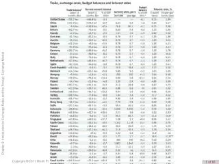
Quarterly percentage changes in nominal exchange rates and relative prices, UK
Judging PPP • All in all there appears to be evidence – both empirical and theoretical – to justify a departure from strict PPP theory. • The conventional wisdom is that as a theory, PPP is most useful and realistic in the longer term. • In the short run, the nominal exchange rate is much more volatile than the theory of PPP would imply. This can be taken as an indication that there may be other factors which drive the nominal exchange rate. The theory of Purchasing Power Parity predominately relates to the trade in physical goods and services, but these current account trades only make up a small part of the overall balance of payments.
UIP: Uncovered Interest Parity • Given that much of the capital account constitutes short-term financial flows, it may also account for the observed volatility in short term exchange rates. • Whereas PPP determines the exchange rate to arbitrage prices in the goods market, Uncovered Interest Parity (UIP) does a similar thing in the financial assets market. • Since the 1980s, liberalisation in the world’s financial markets means that currency transactions related to the trade in financial assets outweighs that in goods and services by as much as 100:1 in value terms. • Much of this is very liquid and can move around the world at great speeds in search of the best returns. • Uncovered Interest Parity (UIP) models the exchange rate through relative asset returns.
UIP: Uncovered Interest Parity • The two key assumptions in this model are that assets are perfectly substitutable, and there is perfect international capital mobility. As a result, arbitrage means that the exchange rate will change so that the returns on all financial assets should be equalised. • When you purchase a foreign asset, there are two things that determine the returns that are derived from it: • The overseas interest rate is defined by r*. • Exchange rate movements, E. • The first of these is clear. The second refers to having purchased a foreign asset, the returns are only realised once they have been converted back into domestic currency. If, however, the exchange rate changes, the rate at which this conversion takes place will also change.
UIP: Uncovered Interest Parity • The overall returns from investing overseas will be equal to both the foreign interest rate and also the interim percentage change in the exchange rate: • The theory of UIP is based on the idea that the expected returns from investing in domestic and foreign assets should be equalised. r = r* + %E, • Rearranging, = r – r* • This is the UIP condition: the expected change in the exchange rate is equal to the differential between domestic and foreign interest rates.
UIP: Uncovered Interest Parity • Under rational expectations, people on average form correct expectations of the change in the exchange rate so: • If the domestic interest rate rises above (falls below) the foreign rate, then there will be an expectation of a depreciation (an appreciation) in the exchange rate.
UIP: Uncovered Interest Parity • The best approach to explaining how UIP works is through a very simple example. • Suppose that initially the domestic and foreign interest rates were equal. In this case, international investors are indifferent between the domestic and foreign assets, and there is no expected change in the exchange rate. • However, the domestic interest rate then rises by 2% for one period, after which it returns to its original level. • Now that domestic assets offer higher returns, the demand for foreign currency will fall as domestic investors substitute out of foreign and into domestic assets. The supply of foreign currency will also increase as foreign investors do the same. • Consequently, the domestic exchange will appreciate from E1 to E2.
UIP: Uncovered Interest Parity • However, once that interest differential disappears, what should happen to the exchange rate? • As domestic assets are no longer offering higher returns than on foreign assets, there is no reason for the demand and supply curves to stay at D2 and S2, respectively. Both will return to their initial levels and the exchange rate will return to E1. • The initial appreciation in the exchange rate will only last as long as the interest differential is expected to persist.
UIP: Uncovered Interest Parity • However, by how much will the domestic exchange rate appreciate (E1 to E2)? • Well, according to the UIP condition, this will be by 2%. We know that once the interest rate falls back to its initial value, the exchange rate must return to its initial value. Therefore, this immediate appreciation must be stimulating expectations of a depreciation, and from UIP, this expected depreciation will be 2%. • So, in order to depreciate 2% back to its initial value, the exchange rate must first of all appreciate by the same – exactly 2%. This is shown in the next figure.
UIP: Uncovered Interest Parity • The movements in the exchange rate act to equalise the returns on domestic and foreign assets, just as UIP predicts. Although domestic assets offer 2% more than those abroad, this is countered by the expected 2% depreciation in the currency. • What if the exchange rate were to initially appreciate by less than 2%? In this case, the interest differential would be 2%, but the expected depreciation would be less than 2%. Domestic assets would offer higher returns than those overseas, encouraging further purchases of domestic assets would then appreciate the exchange rate further until the appreciation had reached 2%.
UIP: Uncovered Interest Parity • The UIP relationship is effectively maintained by international investors who seek to achieve the highest returns possible. Arbitrage is much stronger here than in the goods market due to the relative ease at moving large sums of finance around the world and due to competition among different investors. If international investors have billions of Pounds at their disposal, then very small interest differentials will lead to significant differences in returns. • This will also explain why exchange rate movements are very fast. In the above figure, the exchange rate effectively jumps as soon as the interest differential appears. This is because any investor who can purchase the domestic assets before the exchange rate has fully appreciated will make additional returns.
UIP: Uncovered Interest Parity • The size of exchange rate changes following interest rate movements depends on both the size and the persistence of interest rate differentials. An one period interest differential is 4%. This would then generate an initial appreciation of the same amount, with of course an expected depreciation of also 4% over the period. • If the interest differential were 2% but was maintained for two periods, then the initial appreciation in the exchange rate would once again be approximately 4%. As the differential is 2% in each period, from the UIP relationship, the expected depreciation in each would also be 2%, justifying the initial appreciation of about 4%. • This is shown in the following figures.
UIP: Uncovered Interest Parity • As a theory accounting for short-term movements in the exchange rate, UIP is important. The following figure plots evidence for the UK-U.S. nominal exchange rate. There is cursory evidence to suggest that an appreciation in the exchange rate is associated with a positive interest differential. • There are though two extensions to the theory of UIP, which might break the relationship between short-term exchange rate movements and the interest differential. • The first is the idea that there are different risks in investing in different assets. Secondly, interest-bearing assets are not the only financial assets; there are also equities and the currencies themselves. Accepting a wider definition of what constitutes a financial asset might explain exchange rate movements.
Risk Premia • Therefore, the UIP condition may work better if it is adapted to include a risk premium: • where μ is the relative risk premium on domestic assets. • A positive interest differential can no longer be taken as an indicator that the currency will appreciate (generating the expectation of a depreciation). • If the risk premium is relatively large, then the risk adjusted interest differential may in fact be negative – leading to a depreciating exchange rate (an expectation of an appreciation).
Stock Markets and the Exchange Rate • In reality, investing overseas does not always need to be in the form of interest bearing assets, such as bonds or bank accounts. Equity investments normally take the form of assets such as stocks and shares. • It should certainly be apparent from the next figure that in a short horizon exchange rates are very volatile and displays the same type of random walk process that describes financial markets. • As financial asset prices are based on expected future profits, prices will jump every time new information is revealed to the market. As information is always arriving at markets, share prices will be volatile and this is reflected in currency markets.
Stock Markets and the Exchange Rate • There is a strong linkage between stock and currency markets. For example, suppose new information comes to light predicting a downturn in the U.S. economy. The expectation of lower future profits will place downward pressure on equity prices and investors will sell, perhaps transferring funds into Japanese or European assets. The $US will subsequently depreciate. • Longer-term volatility relationships can also be accounted for, e.g., the sharp appreciation in the $US during the late 1990s and the U.S. asset bubble in U.S. • The relationship between stock markets and currencies can also cloud the UIP relationship. Increases in interest rates need not always lead to an appreciation in the exchange rate. In fact, a rise in interest rates would be expected to lead to a fall in stock market prices and may therefore lead to a depreciation in the exchange rate.
Currency Trading • Explaining exchange rate volatility is even easier once we allow for the fact that the exchange rate itself can be viewed as the price of a financial asset. This is because currency traders aim to make money by predicting the movements in the exchange rate. • For example, at one moment in time, a trader could purchase on the spot market. If the domestic currency then depreciates, the domestic currency can then be repurchased and a profit made. • When currencies themselves are viewed as financial assets, it means that they too can be subject to the same volatility as other financial assets. This is certainly true in the short run, but may also manifest itself in long-term volatility, such as bubbles. The long appreciation in the $US at the beginning of the 1980s is certainly an example.