Download
1 / 28
290 likes | 477 Views
Molecular dynamics in the microcanonical (NVE) ensemble: the Verlet algorithm. Javier Junquera. Equations of motion for atomic systems in cartesian coordinates. Classical equation of motion for a system of molecules interacting via a potential.

E N D
Molecular dynamics in the microcanonical (NVE) ensemble:the Verlet algorithm Javier Junquera
Equations of motion for atomic systems in cartesian coordinates Classicalequation of motionfor a system of moleculesinteractingvia a potential Thisequationalsoapliestothe center of massmotion of a molecule, withtheforcebeginthe total externalforceactingonit
Hamilton or Lagrange equations of motion Lagrange’sequation Hamilton’sequations To compute the center of masstrajectoriesinvolvessolving… A system of 3Nsecondorderdifferentialequations Oranequivalent set of 6Nfirst-orderdifferentialequations
Hamilton or Lagrange equations of motion Lagrange’sequation Hamilton’sequations To compute the center of masstrajectoriesinvolvessolving… A system of 3Nsecondorderdifferentialequations Oranequivalent set of 6Nfirst-orderdifferentialequations
Conservation laws Assumingthat and do notdependexplicitlyon time, so that Essentialcondition: No explicitly time dependentorvelocitydependentforceacting Then, the total derivative of theHamiltonianwithrespectto time FromtheHamilton’sequation of motion TheHamiltonianis a constant of motion Independent of theexistence of anexternalpotential
The equations are time reversible Bychangingthesigns of allthevelocities and momenta, wewill cause themoleculestoretracetheirtrajectories. Iftheequations of motion are solvedcorrectly, thecomputer-generatedtrajectorieswillalsohavethisproperty
Standard method to solve ordinary differential equations: the finite difference approach Given molecular positions, velocities, and otherdynamicinformation at a time h=t Notes: t0 t1 t2 tn-1 tn tn+1 tN Theequations are solvedon a stepbystepbasis Thechoice of the time intervalwilldependonthemethod of solution, butwill be significantlysmallerthanthetypical time takenfor a moleculetotravelitsownlength Weattempttoobtainthe position, velocities, etc. at a later time , to a sufficientdegree of accuracy
General step of a stepwise Molecular Dynamics simulation Predict the positions, velocities, accelerations, etc. at a time , using the current values of these quantities Evaluate the forces, and hence the accelerations from the new positions Correct the predicted positions, velocities, accelerations, etc. using the new accelerations Calculate any variable of interest, such as the energy, virial, order parameters, ready for the accumulation of time averages, before returning to the first point for the next step
Desirable qualities for a successful simulation algorithm Itshould be fast and requirelittlememory Sincethemost time consumingpartistheevaluation of theforce, therawspeed of theintegrationalgorithmisnot so important It should permit the use of long time step Far more importanttoemploy a long time step. In thisway, a givenperiod of simulation time can be covered in a modestnumber of steps Itshouldduplicatetheclassicaltrajectory as closely as possible It should satisfy the known conservation laws for energy and momentum, and be time reversible It should be simple in form and easy to program Involvethestorage of only a fewcoordinates, velocitites,…
Desirable qualities for a successful simulation algorithm Itshould be fast and requirelittlememory Sincethemost time consumingpartistheevaluation of theforce, therawspeed of theintegrationalgorithmisnot so important It should permit the use of long time step Far more importanttoemploy a long time step. In thisway, a givenperiod of simulation time can be covered in a modestnumber of steps Itshouldduplicatetheclassicaltrajectory as closely as possible It should satisfy the known conservation laws for energy and momentum, and be time reversible It should be simple in form and easy to program Involvethestorage of only a fewcoordinates, velocitites,…
Energy conservation is degraded as time step is increased ECONOMY ACCURACY Allsimulationsinvolve a trade-off between A good algorithm permits a large time step to be used while preserving acceptable energy conservation
Parameters that determine the size of • Shape of thepotentialenergy curves • Typical particle velocities Shorter time steps are used at high-temperatures, for light molecules, and forrapidlyvaryingpotentialfunctions
The Verlet algorithm method of integrating the equations of motion: description of the algorithm Method based on: - the positions - the accelerations - the positions from the previous step Direct solution of the second-order equations A Taylor expansion of the positions around t Adding the two equations
The Verlet algorithm method of integrating the equations of motion: some remarks Remark 1 The velocities are not needed to compute the trajectories, but they are useful for estimating the kinetic energy (and the total energy). They can be computed a posteriori using [ can only be computed once is known] Remark 2 Whereas the errors to compute the positions are of the order of The velocities are subject to errors of the order of
The Verlet algorithm method of integrating the equations of motion: some remarks Remark 3 The Verlet algorithm is properly centered: and play symmetrical roles. The Verlet algorithm is time reversible Remark 4 Theadvancement of positions takes place allin onego, ratherthan in twostages as in the predictor-corrector algorithm.
The Verlet algorithm method of integrating the equations of motion: overall scheme …and we repeat the process computing the forces (and therefore the accelerations at ) Known the positions at t, we compute the forces (and therefore the accelerations at t) Then, we apply the Verlet algorithm equations to compute the new positions
Molecular Dynamics Timestep must be small enough to accurately sample highest frequency motion Typical timestep is 1 fs (1 x 10-15 s) Typical simulation length: Depends on the system of study!! (the more complex the PES the longer the simulation time) Is this timescale relevant to your process? Simulation has two parts equilibration – whenproperties do notdependon time production (record data) Results: diffusion coefficients Structural information (RDF’s,) Free energies / phase transformations (very hard!) Is your result statistically significant?
How to run a Molecular Dynamic in Siesta: the Verlet algorithm (NVE-microcanonical ensemble)
Computing the instantaneous temperature, kinetic energy and total energy
How to run a Molecular Dynamic in Siesta: the Verlet algorithm (NVE-microcanonical ensemble) Maxwell-Boltzmann
SystemLabel.MDE Output of a Molecular Dynamic in Siesta: the Verlet algorithm (NVE-microcanonical ensemble) Conservedquantity Examplefor MgCoO3 in therhombohedralstructure
Output of a Molecular Dynamic in Siesta: SystemLabel.MDAtomic coordinates and velocities (and lattice vectors and their time derivatives if the dynamics implies variable cell). (unformatted; post-process with iomd.F) SystemLabel.MDE shorter description of the run, with energy, temperature, etc. per time step SystemLabel.ANI(contains the coordinates of every Molecular Dynamics step in xyz format) These files are accumulativeevenfordifferentruns. Remembertodeletepreviousonesifyou are notinterestedonthem
Check conservation of energy Length of time step: 3 fs $ gnuplot $ gnuplot> plot "md_verlet.MDE" using 1:3 withlines, "md_verlet.MDE" using 1:4 withlines Compare: Total energy with KS energy $ gnuplot> set terminal postscript color $ gnuplot> set output “energy.ps” $ gnuplot> replot
Check conservation of energy Length of time step: 1 fs $ gnuplot $ gnuplot> plot "md_verlet.MDE" using 1:3 withlines, "md_verlet.MDE" using 1:4 withlines Compare: Total energy with KS energy $ gnuplot> set terminal postscript color $ gnuplot> set output “energy.ps” $ gnuplot> replot
Check conservation of energy Length of time step: 0.5 fs $ gnuplot $ gnuplot> plot "md_verlet.MDE" using 1:3 withlines, "md_verlet.MDE" using 1:4 withlines Compare: Total energy with KS energy $ gnuplot> set terminal postscript color $ gnuplot> set output “energy.ps” $ gnuplot> replot
Check conservation of energy Length of time step: 0.1 fs $ gnuplot $ gnuplot> plot "md_verlet.MDE" using 1:3 withlines, "md_verlet.MDE" using 1:4 withlines Compare: Total energy with KS energy $ gnuplot> set terminal postscript color $ gnuplot> set output “energy.ps” $ gnuplot> replot
Visualisation and Analysis Molekel http://www.cscs.ch/molekel XCRYSDEN http://www.xcrysden.org/ GDIS http://gdis.seul.org/