Lecture 40: Review of Controls

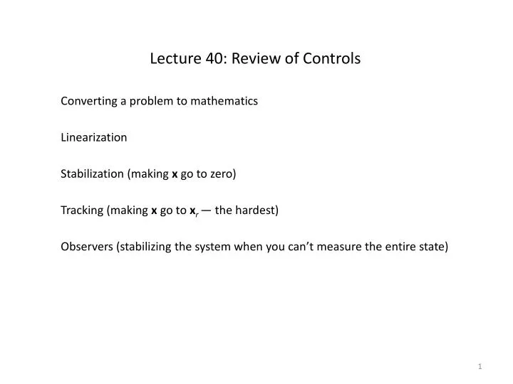
Lecture 40: Review of Controls Converting a problem to mathematics Linearization Stabilization (making x go to zero) Tracking (making x go to xr— the hardest) Observers (stabilizing the system when you can’t measure the entire state)

Converting a problem to mathematics You can write the physics using free body diagrams or the Euler-Lagrange method There may be an auxiliary electrical equation Let’s recall magnetic suspension; it has a number of useful features.

Converting a problem to mathematics yis positive down Numerical parameters for later

Converting a problem to mathematics We’ll need to convert the second order dynamical equation to a pair of first order equations We’ll want to rearrange the electrical equation to look like a state equation Our state vector will be where v denotes the rate of change of y

Converting a problem to mathematics Manipulate the equations combine these input

Converting a problem to mathematics and I have replaced e by the generic input variable u This is a nonlinear problem, which brings us to the next step

Linearization We linearize about some reference state, some point in state space that is stationary This is frequently, but not always, zero For the magnetic suspension system is it not zero The reference state may include a reference input, as it does for the magnetic suspension

Linearization Find the reference state We have Clearly v0 = 0. y0 cannot be zero, so we have Finally

Linearization We are at liberty to select one of these variables. y0 makes the most sense. The reference state is then We get the linear equations by writing x = x0 + x’, e = e0 + e’

Linearization One way, the brute force and awkwardness way, is to substitute for x and e and expand all the terms, keeping only those linear in the primed variables This works if the problem is simple, and it can be done if the problem is hard The better way is to differentiate the nonlinear force F

Linearization Linearization by differentiation Think of expanding F in a three variable Taylor series around the equilibrium

Linearization substitute the equilibrium values

Linearization Remember that So that the expressions become And these are the columns of the linearized matrix

Linearization Let’s look at another example of linearization by differentiation Find an equilibrium such that this vanishes and linearize about that equilibrium

Linearization Take the simple equilibrium, for which x = 0

Linearization The more complicated equilibrium is In this case we have

QUESTIONS?

Stabilization We have arrived at the canonical problem where our goal is to choose u in such a way that x will go to zero We do that using full state feedback, setting u = -gx We need to findg, and we have a ritual to do that The ritual only works if the system is controllable and the first step in the ritual is figuring out if the system is controllable. It’s probably worth noting that: A is a kxk square matrix gis a kx 1 column vector bis a 1 xk row vector

Stabilization Step one is to form the controllability matrix and calculate its determinant. If the determinant is nonzero the system is controllable and we can move forward Find the inverse ofQand select its last row This is a row vector. We calculate k – 1 more rows to make a square matrix T.

Stabilization And we have the square matrix which is invertible We use T to do a change of variable (which just amounts to a change of basis for the mathematically inclined of you) We see what happens on the next slide

Stabilization We can multiply this last equation by T to get We agree to rename the matrices and vectors to make this equation A1 and B2 are in companion form; here’s a k = 6 example

Stabilization Now we are ready to talk about gains, and we have to start in terms of z x will go to zero if z goes to zero. z will go to zero if the eigenvalues of Ac all have negative real parts. We call these eigenvalues poles. Because of the companion form, it is easy to choose gains to put the poles where we want them

Stabilization The k = 6 example The characteristic polynomial Remember this ritual for finding characteristic polynomials You don’t need to calculate determinants

Stabilization We can form the characteristic polynomial for the poles we want Expand that in powers of s and equate the coefficients to determine the gains (in z space) Once we have those, we need to go back tox space, and let’s see how that goes

Stabilization Were there but worlds enough and time I would now have you work a stabilization problem But there ain’t, so I’ll work one

Stabilization The inverse: swap the diagonal terms change the signs of the off-diagonal terms divide by the determinant Build T

Stabilization The inverse: swap the diagonal terms change the signs of the off-diagonal terms divide by the determinant The companion forms

Stabilization Now we can form Ac and work on its eigenvalues (the poles) Characteristic polynomials

Stabilization The choice of poles is up to you Critical damping: s1 = -r = s2 Conjugate pair: s1 = -r+ jq , s2 = -r- jq

QUESTIONS?

Tracking This is probably the hardest one, and we haven’t spent much time on it Find some ur such that Find some Arsuch that Two options present themselves to us: We found the second method to work better in the one problem we did with both

Tracking We compare with Friedland equation (6.37)

Tracking We can ask that the derivative of the error goes to zero, from which is stable, hence invertible and we can write the latter form being equivalent to equation 6.40 We find g in the same manner we just rehearsed

Tracking It may happen that we can actually make e vanish in its entirety If that is the case, then we will be very happy It is more generally true that we cannot that all we can make vanish is some subset of e typically the part that looks like an error in y This is what Friedland does, multiplies the error by the matrix/vector C For SISO systems, it is the vector c, I’ll leave it a vector for now

Tracking rearrange we want this to work for any xr so . . .

Tracking Let’s look at another 2 x 2 system and see if we can make it track

Tracking From the earlier part of this lecture, we can find the gains given the poles I will take them to be at -1, giving me a critically damped system

Tracking We can build the error matrix and in this case we can actually kill all the error by choosing We select the feedback as we had before

Tracking We can plug all this in and integrate numerically. Here’s the result for Y = 1, w = 2

QUESTIONS?

Observers This last bit depends on the Lecture 38 (and I’m sticking to a single output) Suppose that all we know is an output y, a scalar for an SISO system

Observers We use y, the control and an artificial dynamical system to find an estimate for x and we select the carat matrices to minimize the difference between x and its estimate.

Observers As usual we want to construct a system for the evolution of the error and, of course, make the error go to zero Note that k is a column vector We eliminate the explicit appearance of the estimate

Observers e will go to zero if I get rid of the contributions from x and u and make sure the new matrix is stable This becomes a pole placement exercise

Observers The substitutions give and the error will vanish of the eigenvalues have negative real parts. We need to find k such that this is so. We have two questions: Is this possible? How?

Observers For our SISO system the K vector is a column and the system looks like We can make this look like something we already know how to do by taking the transpose The eigenvalues of the transpose of a matrix are the same as those of the original matrix

Observers cT looks like b and kT looks like g We have the analog of the controllability theorem The observability theorem We can build an observer if det(N) ≠ 0.

Observers

Observers Let’s apply this to a simple model problem I will skip the calculation of the regular gain matrix, because we’ve just gone through one The result is

Observers

Lecture 40: Review of Controls