Download
1 / 32
320 likes | 344 Views
Mesh Control using Size Functions and Boundary Layers. Size Functions and Boundary Layers. Size functions and boundary layers are mesh control tools available in GAMBIT. Size functions

E N D
Size Functions and Boundary Layers • Size functions and boundary layers are mesh control tools available in GAMBIT. • Size functions • Can be used to smoothly control the growth in mesh size over a particular region of the geometry starting from a “source,” or origin. • Can also be used to smoothly transition from fine mesh needed to resolve flow physics, curved geometry and model flow in thin gaps. • Boundary layers • Used to grow layers of cells of desired height from specified boundaries of 2D/3D geometry • Typically used to capture near wall phenomena such as turbulence and heat transfer. • Multiple size functions and boundary layers can be used to control mesh size distribution.
Size Functions • Size functions control the mesh distribution in a region of space, including edges, faces, and volumes similar to the way grading controls mesh distribution on edges. • Size functions are accessed through the Tools menu. • Size functions are designed to grade tetrahedral meshes even though they can be used with a hex mesh. Curvature size function refines the mesh in regions of large curvature Proximity size function ensures a fine mesh in small gaps. Multiple Size Functions: Curvature and Proximity
Types of Size Functions • Size functions require the specification of the type, source entities, attachment, and size parameters. • The type of size function dictates the criteria upon which the mesh will grow. • Fixed – scope is a fixed region about a source. • Curvature – scope is a region near highly curved surfaces. • Proximity – scope is a region within a specified distance from objects. • Meshed – ensures that a mesh is propagated in a controlled manner from premeshed boundaries of the domain.
Size Function Definition • Each size function type requires specification of: • Source entities • Defines the shape and location of the "origin" of the affected region. • Attachment entities • Host the mesh that will be affected. • Parameters • Three parameters define the characteristics of the size function (except the meshed size function) • The two parameters common to all four size function types are the growth rate and size limit. • The third (initialization) parameter is different for each of the first three size function types. • The meshed size function does not use an initialization parameter.
Selecting the Source Entity • Source • Can be vertices, edges, faces, or volumes • Can be internal or external to attachment entities • Source entity defines shape of scope
Selecting the Attachment Entity • The attachment entities host the mesh that is to be affected
No Size Function (3,684 cells) Fixed Size Function (1,730 cells) Fixed Size Function • Parameters • Start size: Mesh size adjacent to the source entity • Growth rate: Size ratio of two adjacent mesh elements • Size limit: Maximum allowable mesh size on attachment entity Same edge mesh (50 intervals) Attachment: face Source: edge
Large angle Small angle Curvature Size Function • Parameters • Angle: The maximum allowable angle between outward pointing normals for any two adjacent mesh elements. • Growth rate and Size limit – same as for fixed S.F. Without Curvature S.F. With Curvature S.F.
Proximity Size Function • Specifies number of cells in face gap (3D) and edge gap (2D) • For 3D gaps, the pair of faces bounding the gap are specified as source entities. • For 2D gaps, the pair of edges bounding the gap or the face containing the gap can be specified as sources. • If a volume is selected as the source, then all pairs of faces will be evaluated as possible 3D gaps. • Parameters • Cells per gap: number of mesh layers in the gap • Growth rate and Size limit: same as for fixed • Limitations • Becomes slow on large models • Improper use may result in abrupt change in size • Solution – increase resolution by changing the defaults for background grids • Proximity size functions are useful for both quad pave and tri meshes in 2D and tet meshes in 3D Gap defined by two source faces
Meshed Size Function • The mesh is grown from the meshed source entities into the attachment entity. • Parameters: • No initialization parameter is needed. • Growth rate and size limit need to be specified. • Limitations • The source entities must be premeshed. Premeshed source edges Premeshed source face
Size Function Utilities • Modify Size Function • Size function input parameters can be modified after the size function has been created. • Source and Attachment entity list • Size and Growth Rate • You must press Apply for the changes to be made.
Size Function Utilities • View Size Function • Select the size function to view • Click the Initialize button • Use the slider bar to view the range of influence in the graphics window. Initialized size function on aircraft wing
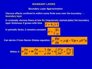
Boundary Layers • Boundary layers are layers of elements growing outward from a boundary into the domain. • Produces high quality cells near the boundary. • Allows resolution of flow field effects with fewer cells than would be required without them. • In general, boundary layers are attached to: • Edges for 2D problems • Faces for 3D problems High quality boundary layer mesh
Defining a Boundary Layer Algorithm Definition Input Settings Transition Pattern Attachment Entities
Boundary Layer Algorithms • Three boundary layer algorithms are available: • Uniform • Aspect Ratio (first) • Aspect Ratio (last) Uniform Aspect Ratio (first) row Aspect Ratio (last) row Adjacent cells have the same height Adjacent cells have the same aspect ratio Cells in the last layer have the user-prescribed aspect ratio Aspect ratio is constant within each layer of cells Aspect ratio of the last layer is specified. Height is constant within each layer of cells
Boundary Layer Inputs • Uniform boundary layer – The first three inputs are required; the fourth is calculated) • First row Height of first row of elements (a) • Growth factor Factor for geometric series (b/a) • Rows Total number of layers • Depth Boundary layer thickness (D) • Aspect ratio-based boundary layer inputs are similar • First percent Starting aspect ratio • Growth factor Factor for geometric series (b/a) • Number of rows • For aspect ratio (last), inputs are First Row, Number of Rows, and Aspect ratio of last layer.
ON (No Overlap at Corner) OFF (Overlap at Corner) Internal Continuity Option • The Internal Continuity option allows 3D boundary layers to be formed with no crossover or overlap regions.
Wedge Corner Shape Option • The Wedge Corner Shape option is used at corner or reverse vertices to create a rounded “wedge” of elements for 2D Boundary Layers. ON (Wedge Shape) OFF (Block Shape)
Boundary Layer Attachments • 2D boundary layers are attached to edges. • 3D boundary layers are attached to faces. • Temporary Display • A boundary layer is initially displayed in orange to indicate that it is temporary. • Display updates immediately when changes are made. • Direction arrow • Points from the attachment entity toward the centroid of the parent entity. • This can be misleading, especially in 3D! • The boundary layer is displayed in white (permanent) after clicking Apply.
View 3D Boundary Layers • The View 3D Boundary Layers tool allows users to examine a 3D boundary layer mesh prior to volume meshing. • Resolves many mesh quality issues • Resolves tet mesh failure
Boundary Layers and Vertex Types E • 2-D Boundary layers in regions near vertices are defined by the vertex type. • End: mesh overlaps • Corner: angle trisected • Reverse: angle divided into fourths. • Side: angle bisected • The vertex type for Boundary Layers can be changed in the Set Face Vertex Form in the Face meshing menu with the Boundary layer only option turned on. • Vertex types are also important for imprinting 3D boundary layers on adjacent faces. E E E R C E E S E
Imprinting Adjacent Faces with 3D Boundary Layers • A 3D boundary layer attached to a face may imprint the adjoining faces, depending on the vertex type of the vertices at the intersection of the boundary layer attachment face and adjoining faces. • If the vertex is an “End” type vertex, an imprint is created and displayed. • If 3D boundary layers are also attached to the adjoining faces, then the Internal Continuity toggle will determine the crossover region and imprint. Imprint of 3D boundary layer on adjacent faces with 3D boundary layer attached to bottom face
140° E E E Imprinting 3D Boundary Layers by Modifying Vertex Types • When the angle between adjacent and attachment faces in greater than 120°, a vertex type change to End can cause the 3D boundary layer to imprint. Attachment face No imprinting of 3D boundary layer and gaps due to side vertices at the face intersections Vertex types changed to End closes the gap and imprints 3D boundary layer
How Do Size Functions Work? • Size functions work by generating a discrete map of mesh size on a background Cartesian grid that overlays the attachment geometry. • This map is used by the meshing algorithms in growing mesh with a size distribution. • Multiple size functions can be integrated into a single global size function on the entire domain. • Size functions work in two steps: • Size function initialization wherein a size distribution is computed on the source entities. • Background grid generation on the attachment entity, which resolves the variation of the mesh size as a function of the distance from the source. entity. Typical background grid for an automotive manifold
How Do Size Functions Work? • Size function initialization: • A constant “fixed” mesh size is used for the fixed size function. • For the curvature size function and proximity size functions, the source entity is successively divided into smaller “facets” and a size is computed on each facet. • Each facet meets the angle criterion for the curvature size function. • Each facet meets a criterion on the gap distance between opposite facets for the proximity size function. • This can be computationally intensive for complex surfaces. • The Initialize Size Function button allows you to visualize the size function variation radiating from the source entity. Initialized size function on aircraft wing
Sc – (Savg) > (tolerance) How Do Size Functions Work? • Background grid generation: • A set of Cartesian boxes forming a grid that bounds the attachment geometry are generated and refined into smaller boxes. • This successive refinement of the background grid is carried out until a maximum number of levels of refinement (or “tree depth”) is reached or the size variation in all boxes is less than a specified tolerance. • Background grid refinement: • A size is calculated in each box at the nodes and the center, as a function of the distance from the source entity. • The box is divided along the X,Y and Z axes If the size at the center is greater than the average of the size at the nodes by a tolerance (nonlinear error percent). S1 S2 SC S3 S4 Source entity Boundary of attachment entity Refined background grid
Background Grid Generation • Use of the background grid default parameters is key to obtaining the desired meshes! • TOOLS.SFUNCTION.BGRID_MAX_TREE_DEPTH controls the maximum refinement of the background grid • Increase the default value (16 in GAMBIT 2.2) until no cells hit the tree depth. • A value of –1 puts no limit on the background tree depth, but makes size functions too slow for large models • TOOLS.SFUNCTION.NONLINEAR_ERR_PERCENT controls the allowable deviation of the local mesh from the prescribed mesh size • Default is 25%, can vary between 3 and 25% • Number of cells above the prescribed tolerance are reported in the transcript window • TOOLS.SFUNCTION.REPORT_BGRID_INFO = 1 turns reporting in the transcript window on.
Increasing Background Tree Depth Background grid level reached maximum value specified Size Function not sufficiently resolved Ideal background grid Underresolved Background Grid Resolved Background Grid
Boundary Layer Defaults • GAMBIT defaults set values for the critical parameters for growing boundary layers. • Knowledge of the important defaults will help control the mesh on complex 2D and 3D geometry. • Boundary layer defaults are available in the BLAYER and BLAYERTGRID sections under the Mesh tab in the Edit Defaults form. Edit → Defaults… • The GAMBIT Command Reference Guide provides more information on defaults.