Download
1 / 26
260 likes | 598 Views
Resolving Clouds in Atmospheric Models Bill Skamarock NCAR/MMM Clouds in the Atmosphere Weather: Precipitation – rain, snow, hail Wind, radiation, visibility Chemistry/Air-Quality: Chemical processing (acid rain) Ozone chemistry Transport of pollutants

E N D
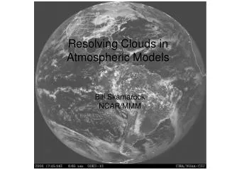
Resolving Clouds in Atmospheric Models Bill Skamarock NCAR/MMM
Clouds in the Atmosphere Weather: Precipitation – rain, snow, hail Wind, radiation, visibility Chemistry/Air-Quality: Chemical processing (acid rain) Ozone chemistry Transport of pollutants Wet deposition Climate Moisture redistribution and precipitation – hydrological cycle Radiation
Representation of Clouds in Atmospheric Models Large-scale models: h > 30 km • The effects of the clouds are diagnosed (parameterized) from • the predicted water vapor field • precipitation • vertical transport and redistribution of moisture and heat • radiative effects • turbulence
Representation of Clouds in Atmospheric Models Meso-scale models: 8 km < x < 30 km • The effects of the clouds are partially prognosed from • predicted fields: water vapor, cloud water and ice, and frozen • and liquid precipitation. • Some portions of the cloud effects are still diagnosed (parameterized). • some precipitation • some vertical transport and redistribution of moisture and heat • turbulence
Representation of Clouds in Atmospheric Models Cloud-scale models: 100 m < x < 8 km The effects of the clouds are entirely prognosed from predicted fields: water vapor, cloud water and ice, and frozen and liquid precipitation.
Problems with Modeled Clouds Large-scale models (clouds completely diagnosed): Poor diagnosis of cloud type, composition, and precipitation. Clouds and cloud-systems do not know about vertical wind shear. Implications: (1) Large uncertainty in climate-model predictions (2) A key limiting factor for weather-forecast accuracy
Meso-/Cloud-Scale Model (WRF) Hurricane Katrina Reflectivity at Landfall 29 Aug 2005 14 Z 4 km WRF, 62 h forecast Mobile AL Radar
Realtime WRF 4 km BAMEX Forecast 12 h forecast Initialized 5/24/03 00Z Reflectivity Forecast Composite NEXRAD Radar
Realtime WRF 4 km BAMEX Forecast 12 h forecast Initialized 5/24/03 00Z Reflectivity Forecast Composite NEXRAD Radar
Vertical Velocity at z = 5 km, t = 5 h Along-line cell spacing ~ 6 to 8 Dh until Dh < 500 m (cell diameter is 3 to 4 km in converged solutions) (Courtesy of G. Bryan, NCAR/MMM)
x = 4000 m Simulations using x = 4 km to x = 250 m x = 1000 m Weak-shear case: Vertical cross-section of tracer concentration at 6 h (not a line-average). x = 250 m (Courtesy of G. Bryan, NCAR/MMM)
Surface rain rate, weak shear 250 m solution close to convergence 1, 2, 4 km solutions over-predict precipitation. (Courtesy of G. Bryan, NCAR/MMM)
Problems with Cloud Models When will our applications get there? (assume comp. speed doubles every 18 months) Climate- not in my lifetime Weather - global (state-of-the-art h ~ 25 km) 36 years (maybe in my lifetime) Weather - regional (state-of-the-art h ~ 7 km) 19 years (hopefully in my lifetime – but will I be retired?) Solutions do not statistically converge until h < O(100 m) - turbulence problem
Cloud Models Cloud models solve the 3D Euler equations and transport equations for water vapor and liquid/solid water species with subgrid models for turbulence and other models (parameterizations) for everything else (moisture phase changes, radiation, land-surface, ocean-surface, etc.) Generally speaking, there are 2 flavors: (1) Semi-Implicit (implicit treatment of acoustic and gravity waves) usually found in global models on lat-long grids – pole problem. (2) Explicit (explicit treatment of acoustic and gravity waves) some form of splitting is usually used to advance acoustic and gravity waves with a shorter timestep.
WRF-ARW • Terrain-following hydrostatic pressure vertical coordinate • Arakawa C-grid • 3rd order Runge-Kutta split-explicit time integration • Conserves mass, momentum, entropy, and scalars using flux form prognostic equations • 5th order upwind or 6th order centered differencing for advection • Limited area (not global) (more info - http://www.mmm.ucar.edu/wrf/users/)
Why Explicit • Explicit time integration with splitting is more efficient than implicit solvers (operations for a given level of accuracy). • Solver needs little tuning for application at different grid resolutions and problem sizes. • Easily parallelized for SM, DM and SM/DM architectures.
Time Integration in ARW 3rd Order Runge-Kutta time integration advance Amplification factor
Time-Split Runge-Kutta Integration Scheme dt is the RK3 timestep acoustic timestep (in this case dt/4)
Time-Split Runge-Kutta Integration Scheme In DM applications: A small amount of data is communicated within each acoustic step.
Time-Split Runge-Kutta Integration Scheme In DM applications: A small amount of data is communicated within each acoustic step. A larger amount is data is communicated after each RK substep.
Single version of code for efficient execution on: Distributed-memory Shared-memory Clusters of SMPs Vector and microprocessors Parallelism in WRF: Multi-level Decomposition Logical domain 1 Patch, divided into multiple tiles Inter-processor communication Model domains are decomposed for parallelism on two-levels • Patch: section of model domain allocated to a distributed memory node • Tile: section of a patch allocated to a shared-memory processor within a node; this is also the scope of a model layer subroutine. • Distributed memory parallelism is over patches; shared memory parallelism is over tiles within patches
Implementation of WRF Architecture Hierarchical organization Multiple dynamical cores Plug compatible physics Abstract interfaces (APIs) to external packages Performance-portable Top-level Control, Memory Management, Nesting, Parallelism, External APIs driver ARW solver Other Solvers Physics Interfaces mediation Plug-compatible physics Plug-compatible physics Plug-compatible physics Plug-compatible physics model Plug-compatible physics WRF Software Framework Overview
Courtesy of J. Michalakes; see http://box.mmm.ucar.edu/wrf/WG2/bench/ for more info
Petascale Computing and Clouds Many effects of clouds on climate and weather are largely unknown/uncertain (observations lacking, models at coarse resolution have poor representation of clouds). Most important problem confronting dynamicists and modelers today. Cloud-resolving (Dh ~ O(100 m)) simulations of cloud systems are needed to understand cloud dynamics and to improve parameterizations - a petascale computing challenge. cloud- mixing eddies cloud systems planetary waves synoptic systems clouds >106 meters 105 - 106 meters 102 - 104 meters meters to 100’s meters
Petascale Computing and Clouds Split-explicit cloud models are easiest to scale to peta-computing - no global data exchange or implicit solver needed, numerics are not scale dependent. We can scale our problems to bigger machines. Questions: What will new machine architectures look like? Will we maintain efficiency with scaling and changes in machine architecture? What code architecture changes will be needed? Other problems: load balancing, analysis, I/O.