Download

1 / 24
240 likes | 374 Views
Re-visiting Conjoint ”How Danish pig producers found the future road to the environmentally concerned Danish consumers” By Lene Hansen and Marcus Schmidt. A case story based on a project carried out for The Danish Bacon & Meat Council. Purpose of the study was to obtain.

E N D
Re-visiting Conjoint • ”How Danish pig producers found the future road to the environmentally concerned Danish consumers” • By Lene Hansen and Marcus Schmidt
A case story based on a projectcarried out forThe Danish Bacon & Meat Council
Purpose of the study was to obtain ... • More knowledge about the driving factors in the demand for organically produced pork • Estimates of the market potential for new alternative pork concepts in general and organic produced pork based on existing organic definition Traditional Danish pigsty Outdoor pigs
Research Design • Pilot phase 1: Cluster analyses based on consumer panel data • Explorative phase 2: 7 extended focus groups with heavy, medium and light consumers of pork • Consolidate phase 3: Internal brainstorming among pork specialists • Conjoint phase 4: Classic full profile conjoint analysis in a national representative 1000 housewives sample • Analysis phase 5: Data analyses - Utility values and cluster analyses
Results from pilot phase 1Cluster analyses • No correlation between household’s consumption of pork and housewife's level of interest in environmental and organic subjects • Heavy, medium and light user segmentation chosen for further qualitative research Non-users - 0,3 mio Heavy users - 0,6 mio Light users - 0,7 mio Medium users - 0,7 mio
Environmental concerns Cookingtraditions Opinions about meat quality Animal welfare Health concerns Declarations Likings Prices -Budgets ? Explorative phase: 7 extended focus groups StandardDanish pork Specialbranded pork Organicpork Ideal pork
Results from explorative phase 2and consolidation phase 3 • 10 important consumer created attributes in connection with pork • 1. Meat quality 3 levels • 2. The pork’s content of fat 4 levels • 3. Declarations 5 levels • 4. Environmentally friendly production 3 levels • 5. Medicine residuals 3 levels • 6. The pig’s welfare 3 levels • 7. Feeding 3 levels • 8. Transportation to slaughterhouses 3 levels • 9. Prices 2 levels • 10. Salmonella 2 levels • Total 34 levels
Conjoint phase 4: The Field Study • Data collection method: • Telephone - Mail - Telephone (TMT) • A random sample of 1,000 persons 18-74 years of age - selected as being responsible for the household’s purchase of convenience goods • Effective contacts 1,626. Approx. 90% accepted to participate (received stimuli material by mail). 1,022 completed interviews
Conjoint phase 4: The Field Study • Flow of questioning: 1. Recruitment by phone and agreement about re-interview 2. Mailing of stimuli material - with detailed description of attributes and levels and 9-26 conjoint profiles 3. Re-interviews (telephone): a. Self-explicated approach: 9 point scales for the 10 attributes and ranking of levels b. Conjoint task: ratings of pig profiles c. Post-measurements: Scalings of buying behaviour and attitudes to organic, environmental and pork related statements
135 Note your evaluation on a 9point scale where 1 means nointerest in buying at all, and 9means very interested in buying 2a Fat inside the pork, no fat layer 3e Normal marking: Type of meat, date of wrapping and durability 6c The pigs go together 10-15 animals on the compulsory pigsty area without straws, with a lot of daylight, but they do not get out due to the competing of disease 9d 30% above normal price
Steps involved in Conjoint AnalysisSettings used in the present study are underscored Preference model: Part worth, vector, ideal point Data Collection Method: Full profile, trade off-tables Survey Instrument: Telephone, face-to-face, mail Technology: Computer aided, paper & pencil Stimulus set Construct: Full factorial, fractional factorial (main effects), Pareto-optimal Master Design: Incomplete Block: BIB, PBIB (balanced, partially bal.)Orthogonal Array: (symmetric/as.) ACA-Designs, etc.
Steps involved in Conjoint AnalysisSettings used in the present study are underscored Stimulus Presentation: Verbal, pictorial (stimulus card), physical product, video-clip, sound Measurement Scale thefor Dependent Variable: Rating, ranking, paired comparisons, constant sum, category assignment Estimation Method: Metric (OLS), non-metric monotone transformations) choice probability based (logit, probit)
Recent Research Contributions • Componential Segmentation, Hybrid Conjoint • Clustering, Segmentation, Market Share Simulation • Self-Explicated Models, Full Profile, ACA • Number of Attributes • Number and Scaling (Wording) of Levels • Optimal Product Line Selection • Optimal Pricing (Dynamic Programming Heuristics) • Constrained Parameter Estimation • Acceptable Designs, Goodness of Fit • Source and further details: Schmidt 1995, European Advances in Consumer Research, Vol. 2 p. 311
Methodological Approach Survey: TMT Telephone-Mail-Telephone (CATI) Exposure: Multiple cue Stimulus card Presentation (verbal + pictorial) Model: Part 1: Self-Explicated Part 2: Full Profile Design: Across blocks: (BIB) Balanced Incomplete Block Design - main effects Within blocks: Symmetric Orthogonal Arrays (i.e. Latin Square) Algorithm: Part worths: Non-metric Estimation Simulation: Share of Preference
Estimation Procedure • Transformational Regression • is an • Alternating Least Squares (ALS) algorithm • that optimises using a • Non-linear Iterative Procedure • with a • Monotonic Transformation • of the dependent variable
Software 1. Bretton Clark Conjoint Designer (design within blocks) 2. SAS PROC TRANSREG (part worths) 3. Sawtooth ACA (marketing/market share simulation) • PROC TRANSREG is developed by the SAS Institute • For solving conjoint and related multivariate problems • Pioneered by F. Young and W. Kuhfield in the late 1980s
Approaching the Problem: Attributes and Levels • Attributes Levels • 1 a b c 3 • 2 a b c d 4 • 3 a b c d e 5 • 4 a b c 3 • 5 a b c 3 • 6 a b c 3 • 7 a b c 3 • 8 a b c 3 • 9 a b c d e 5 • 10 a b 2 • Size of Full Factorial Design: 52 x 4 x 36 x 2 = 145.800 Cells (Profiles) Obviously, a strongly reduced design is needed!
Theoretically, it is possible to construct very powerful designs that allow to test for main effects. • One such design, provided by Bretton ClarksConjoint Designer uses only 50 cards. • One of these 50 profiles might look like this …
Hypothetical Profile • Attribute Level • 1. Meat quality Pork for guests • 2. Fat content Lean pork with layer of fat • 3. Declaration Information on land of origin: Farmer’s and farm’s name, type of meat, date of slaughtering + maturing • 4. Environment Production that live up to the Danish environmental legislation completely • 5. Medicine Guaranteed free from residuals • 6. Welfare Pigs go free inside and outside • 7. Feeding Healthy, natural feeding without growth regulators • 8. Transport Pigs killed at farm before transport to slaughterhouse • 9. Price 15% above normal price • 10. Salmonella Control on salmonella as today • Please indicate preference (1=dislike strongly, 10=prefer strongly)
Unfortunately this profile is too “cue-rich” • The respondent is exposed to information overload 10 cues, some of which are complex, are far too much for one profile • And the respondent must rate 50 such profiles • The problem is not so much the number of profiles, but the number of “cues” (information) appearing on a profile • To prevent information overload the authors decided to limit the number of attributes (cues) appearing on a profile to 4 • Statistically speaking, we are looking for a design involving 10 “treatments” (attributes) but only allowing for 4 simultaneous “treatments” within a cell (profile) • One such design is provided by Cochran and Cox (1957): Plan 11.16
Incomplete Block DesignCochran and Cox Plan 11.16 Attribute number 1 1 1 1 1 1 1 2 2 2 2 3 3 3 4 4 Block I II III IV V VI VII VIII IX X XI XII XIII XIV XV 2 2 2 3 4 5 6 3 4 5 7 5 6 4 5 6 3 3 5 7 9 7 8 6 7 8 8 9 7 5 6 8 4 4 6 8 10 9 10 9 10 10 9 10 10 8 7 9
1 ar = bk 10 x 6 = 15 x 4 = 60 2 t(a-1) = r(k-1) 2 x (10-1) = 6 (4-1) = 18 The design needs to fulfil the following two conditions: • where: • a = number of attributes (here: 10) • r = number of times an attribute appears across blocks (6) • b = number of blocks (15) • k = number of attributes within a block (4) • t = number of times two attributes appear within a block (2)
Incomplete Block DesignCochran and Cox Plan 11.16 Attribute number(number of levels in brackets) Number of profiles Complete Reduced 1 1(3) 1(3) 1(3) 1(3) 1(3) 1(3) 2(4) 2(4) 2(4) 2(4) 3(5) 3(5) 3(5) 4(3) 4(3) Block I II III IV V VI VII VIII IX X XI XII XIII XIV XV 2 2(4) 2(4) 3(5) 4(3) 5(3) 6(3) 3(5) 4(3) 5(3) 7(3) 5(3) 6(3) 4(3) 5(3) 6(3) 3 3(5) 5(3) 7(3) 9(5) 7(3) 8(3) 6(3) 7(3) 8(3) 8(3) 9(5) 7(3) 5(3) 6(3) 8(3) 4 4(3) 6(3) 8(3) 10(2) 9(5) 10(2) 9(5) 10(2) 10(2) 9(5) 10(2) 10(2) 8(3) 7(3) 9(5) (b) 25 16 25 25 25 9 25 16 16 25 25 25 25 9 25 316 (a) 180 108 135 90 135 54 300 72 72 180 150 90 135 81 135 1917
Test of Cross validity Number of profiles Pearson’sCorr. Kendal’sTau b Reduced Complete (a) 180 108 135 90 135 54 300 72 72 180 150 90 135 81 135 1917 (b) 25 16 25 25 25 9 25 16 16 25 25 25 25 9 25 316 (c) .74 .73 .78 .87 .62 .72 .49 .84 .81 .71 .76 .87 .79 .70 .75 .75 (d) .51 .48 .62 .66 .44 .44 .45 .65 .69 .55 .58 .70 .68 .55 .61 .57 Block I II III IV V VI VII VIII IX X XI XII XIII XIV XV