Download

1 / 113
1.17k likes | 1.42k Views
14. PARTIAL DERIVATIVES. PARTIAL DERIVATIVES. As we saw in Chapter 4, one of the main uses of ordinary derivatives is in finding maximum and minimum values. PARTIAL DERIVATIVES. 14.7 Maximum and Minimum Values. In this section, we will learn how to: Use partial derivatives to locate

E N D
14 PARTIAL DERIVATIVES
PARTIAL DERIVATIVES • As we saw in Chapter 4, one of the main uses of ordinary derivatives is in finding maximum and minimum values.
PARTIAL DERIVATIVES 14.7 Maximum and Minimum Values • In this section, we will learn how to: • Use partial derivatives to locate • maxima and minima of functions of two variables.
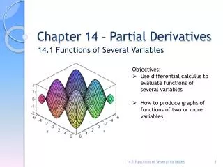
MAXIMUM & MINIMUM VALUES • Look at the hills and valleys in the graph of f shown here.
ABSOLUTE MAXIMUM • There are two points (a, b) where f has a local maximum—that is, where f(a, b) is larger than nearby values of f(x, y). • The larger of these two values is the absolute maximum.
ABSOLUTE MINIMUM • Likewise, f has two local minima—where f(a, b) is smaller than nearby values. • The smaller of these two values is the absolute minimum.
LOCAL MAX. & LOCAL MAX. VAL. Definition 1 • A function of two variables has a local maximumat (a, b) if f(x, y) ≤ f(a, b) when (x, y) is near (a, b). • This means that f(x, y) ≤ f(a, b) for all points (x, y) in some disk with center (a, b). • The number f(a, b) is called a local maximum value.
LOCAL MIN. & LOCAL MIN. VALUE Definition 1 • If f(x, y) ≥ f(a, b) when (x, y) is near (a, b), then f has a local minimumat (a, b). • f(a, b) is a local minimum value.
ABSOLUTE MAXIMUM & MINIMUM • If the inequalities in Definition 1 hold for allpoints (x, y) in the domain of f, then f has an absolute maximum (or absolute minimum) at (a, b).
LOCAL MAXIMUM & MINIMUM Theorem 2 • If f has a local maximum or minimum at (a, b) and the first-order partial derivatives of f exist there, then fx(a, b) = 0 and fy(a, b) = 0
LOCAL MAXIMUM & MINIMUM Proof • Let g(x) = f(x, b). • If f has a local maximum (or minimum) at (a, b), then g has a local maximum (or minimum) at a. • So, g’(a) = 0 by Fermat’s Theorem.
LOCAL MAXIMUM & MINIMUM Proof • However, g’(a) = fx(a, b) • See Equation 1 in Section 14.3 • So, fx(a, b) = 0.
LOCAL MAXIMUM & MINIMUM Proof • Similarly, by applying Fermat’s Theorem to the function G(y) = f(a, y), we obtain: fy(a, b) = 0
LOCAL MAXIMUM & MINIMUM • If we put fx(a, b) = 0 and fy(a, b) = 0 in the equation of a tangent plane (Equation 2 in Section 14.4), we get: z = z0
THEOREM 2—GEOMETRIC INTERPRETATION • Thus, the geometric interpretation of Theorem 2 is: • If the graph of f has a tangent plane at a local maximum or minimum, then the tangent plane must be horizontal.
CRITICAL POINT • A point (a, b) is called a critical point(or stationary point) of f if either: • fx(a, b) = 0 and fy(a, b) = 0 • One of these partial derivatives does not exist.
CRITICAL POINTS • Theorem 2 says that, if f has a local maximum or minimum at (a, b), then (a, b) is a critical point of f.
CRITICAL POINTS • However, as in single-variable calculus, not all critical points give rise to maxima or minima. • At a critical point, a function could have a local maximum or a local minimum or neither.
LOCAL MINIMUM Example 1 • Let f(x, y) = x2 + y2 – 2x – 6y + 14 • Then, fx(x, y) = 2x – 2fy(x, y) = 2y – 6 • These partial derivatives are equal to 0 when x = 1 and y = 3. • So, the only critical point is (1, 3).
LOCAL MINIMUM Example 1 • By completing the square, we find:f(x, y) = 4 + (x – 1)2 + (y – 3)2 • Since (x – 1)2≥ 0 and (y – 3)2 ≥ 0, we have f(x, y) ≥ 4 for all values of x and y. • So, f(1, 3) = 4 is a local minimum. • In fact, it is the absolute minimum of f.
LOCAL MINIMUM Example 1 • This can be confirmed geometrically from the graph of f, which is the elliptic paraboloid with vertex (1, 3, 4).
EXTREME VALUES Example 2 • Find the extreme values of f(x, y) = y2 – x2 • Since fx = –2x and fy = –2y, the only critical point is (0, 0).
EXTREME VALUES Example 2 • Notice that, for points on the x-axis, we have y = 0. • So, f(x, y) = –x2 < 0 (if x≠ 0). • For points on the y-axis, we have x = 0. • So, f(x, y) = y2 > 0 (if y≠ 0).
EXTREME VALUES Example 2 • Thus, every disk with center (0, 0) contains points where f takes positive values as well as points where f takes negative values. • So, f(0, 0) = 0 can’t be an extreme value for f. • Hence, f has no extreme value.
MAXIMUM & MINIMUM VALUES • Example 2 illustrates the fact that a function need not have a maximum or minimum value at a critical point.
MAXIMUM & MINIMUM VALUES • The figure shows how this is possible. • The graph of f is the hyperbolic paraboloid z = y2 – x2. • It hasa horizontal tangent plane (z = 0) at the origin.
MAXIMUM & MINIMUM VALUES • You can see that f(0, 0) = 0 is: • A maximum in the direction of the x-axis. • A minimum in the direction of the y-axis.
SADDLE POINT • Near the origin, the graph has the shape of a saddle. • So, (0, 0) is called a saddle pointof f.
EXTREME VALUE AT CRITICAL POINT • We need to be able to determine whether or not a function has an extreme value at a critical point. • The following test is analogous to the Second Derivative Test for functions of one variable.
SECOND DERIVATIVES TEST Theorem 3 • Suppose that: • The second partial derivatives of f are continuous on a disk with center (a, b). • fx(a, b) = 0 and fy(a, b) = 0 [that is, (a, b) is a critical point of f].
SECOND DERIVATIVES TEST Theorem 3 • Let D = D(a, b) = fxx(a, b) fyy(a, b) – [fxy(a, b)]2 • If D > 0 and fxx(a, b) > 0, f(a, b) is a local minimum. • If D > 0 and fxx(a, b) < 0, f(a, b) is a local maximum. • If D < 0, f(a, b) is not a local maximum or minimum.
SECOND DERIVATIVES TEST Note 1 • In case c, • The point (a, b) is called a saddle point of f . • The graph of f crosses its tangent plane at (a, b).
SECOND DERIVATIVES TEST Note 2 • If D = 0, the test gives no information: • f could have a local maximum or local minimum at (a, b), or (a, b) could be a saddle point of f.
SECOND DERIVATIVES TEST Note 3 • To remember the formula for D, it’s helpful to write it as a determinant:
SECOND DERIVATIVES TEST Example 3 • Find the local maximum and minimum values and saddle points of f(x, y) = x4 + y4 – 4xy + 1
SECOND DERIVATIVES TEST Example 3 • We first locate the critical points:fx = 4x3 – 4yfy = 4y3 – 4x
SECOND DERIVATIVES TEST Example 3 • Setting these partial derivatives equal to 0, we obtain: x3 – y = 0y3 – x = 0 • To solve these equations, we substitute y = x3 from the first equation into the second one.
SECOND DERIVATIVES TEST Example 3 • This gives:
SECOND DERIVATIVES TEST Example 3 • So, there are three real roots: x = 0, 1, –1 • The three critical points are: (0, 0), (1, 1), (–1, –1)
SECOND DERIVATIVES TEST Example 3 • Next, we calculate the second partial derivatives and D(x, y):fxx = 12x2fxy = –4 fyy = 12y2D(x, y) = fxx fyy – (fxy)2 = 144x2y2 – 16
SECOND DERIVATIVES TEST Example 3 • As D(0, 0) = –16 < 0, it follows from case c of the Second Derivatives Test that the origin is a saddle point. • That is, f has no local maximum or minimum at (0, 0).
SECOND DERIVATIVES TEST Example 3 • As D(1, 1) = 128 > 0 and fxx(1, 1) = 12 > 0, we see from case a of the test that f(1, 1) = –1 is a local minimum. • Similarly, we have D(–1, –1) = 128 > 0 and fxx(–1, –1) = 12 > 0. • So f(–1, –1) = –1 is also a local minimum.
SECOND DERIVATIVES TEST Example 3 • The graph of f is shown here.
CONTOUR MAP • A contour map of the function in Example 3 is shown here.
CONTOUR MAP • The level curves near (1, 1) and (–1, –1) are oval in shape. • They indicate that: • As we move away from (1, 1) or (–1, –1) in any direction, the values of f are increasing.
CONTOUR MAP • The level curves near (0, 0) resemble hyperbolas. • They reveal that: • As we move away from the origin (where the value of fis 1), the values of fdecrease in some directions but increase in other directions.
CONTOUR MAP • Thus, the map suggests the presence of the minima and saddle point that we found in Example 3.
MAXIMUM & MINIMUM VALUES Example 4 • Find and classify the critical points of the function • f(x, y) = 10x2y – 5x2 – 4y2 – x4 – 2y4 • Also, find the highest point on the graph of f.
MAXIMUM & MINIMUM VALUES Example 4 • The first-order partial derivatives are:fx = 20xy – 10x – 4x3fy = 10x2 – 8y – 8y3
MAXIMUM & MINIMUM VALUES E. g. 4—Eqns. 4 & 5 • So, to find the critical points, we need to solve the equations 2x(10y – 5 – 2x2) = 0 5x2 – 4y – 4y3 = 0