Download
1 / 37
990 likes | 3.74k Views
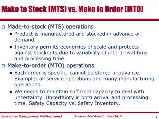
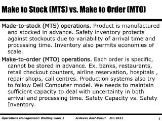
Make to stock vs. Make to Order. Made-to-stock (MTS) operations Product is manufactured and stocked in advance of demand Inventory permits economies of scale and protects against stockouts due to variability of inflows and outflows Make-to-order (MTO) process

E N D
Make to stock vs. Make to Order • Made-to-stock (MTS) operations • Product is manufactured and stocked in advance of demand • Inventory permits economies of scale and protects against stockouts due to variability of inflows and outflows • Make-to-order (MTO) process • Each order is specific, cannot be stored in advance • Process manger needs to maintain sufficient capacity • Variability in both arrival and processing time • Role of capacity rather than inventory • Safety inventory vs. Safety Capacity • Example: Service operations
Examples • Banks (tellers, ATMs, drive-ins) • Fast food restaurants (counters, drive-ins) • Retail (checkout counters) • Airline (reservation, check-in, takeoff, landing, baggage claim) • Hospitals (ER, OR, HMO) • Service facilities (repair, job shop, ships/trucks load/unload) • Some production systems- to some extend (Dell computer) • Call centers (telemarketing, help desks, 911 emergency)
The DesiTalk Call Center TheCall Center Process Sales Reps Processing Calls (Service Process) Incoming Calls (Customer Arrivals) Answered Calls (Customer Departures) Calls on Hold (Service Inventory) Blocked Calls (Due to busy signal) Abandoned Calls (Due to long waits) Calls In Process (Due to long waits)
Service Process Attributes Tp : processing time. Tp units of time. Example, on average it takes 5 minutes to serve a customer. Rp : processing rate. Rp flow units are handled per unit of time. If Tp is 5 minutes. Compute Rp. Rp= 1/5 per minute. Or 60/5 = 12 per hour.
Service Process Attributes Tp : processing time. Rp : processing rate. What is the relationship between Rp and Tp? If we have one resource Rp= 1/Tp In general when we have c recourses What is the relationship between Rp and Tp Rp=c/Tp Each customer always stay for Tp unites of time with the server
Service Process Attributes Tp= 5 minutes. Processing time is 5 minute. Each customer on average is with the server for 5 minutes. c = 3, we have three servers. Processing rate of each server is 1/5 customers per minute. Or 12 customer per hour. Rp is the processing rate of all three servers. Rp = c/Tp Rp= 3/5 customers/minute. Or 36 customers/hour.
Service Process Attributes Ta:customer inter-arrival time. On average each 10 minutes one customer arrives. Ri:customer arrival (inflow) rate. What is the relationship between Ta and Ri Ta = every ten minutes one customer arrives How many customers in a minute? 1/10; Ri = 1/Ta= 1/10 Ri = 1/10 customers per min; 6 customers per hour Ri = 1/Ta
Service Process Attributes Ri MUST ALWAYS <= Rp We will show later that even Ri=Rp is not possible Incoming rate must be less than processing rate Throughput = Flow Rate R= Min (Ri, Rp) Stable Process = Ri< Rp,, so that R= Ri Safety Capacity Rs = Rp– Ri
Operational Performance Measures Waiting time in the servers (processors)? Throughput? Flow time T = Ti+ Tp Inventory I = Ii + Ip Ti: waiting time in the inflow buffer Ii: number of customers waiting in the inflow buffer
Service Process Attributes = Utilization = inflow rate / processing rate = throughout / process capacity = R/ Rp < 1 Safety Capacity = Rp– R For example , R = 6 per hour, processing time for a single server is 6 min Rp= 12 per hour, =R/ Rp = 6/12 = 0.5 Safety Capacity = Rp– R = 12-6 = 6
Operational Performance Measures Given a single server. And a utilization of r = 0.5 How many flow units are in the server ? • Given 2 servers. And a utilization of r = 0.5 • How many flow units are in the servers ?
Operational Performance Measures R • Flow time T Ti+ Tp • Inventory I = Ii + Ip Ip= R Tp I = R T Ii = R Ti R = I/T = Ii/Ti = Ip/Tp Tp if 1 server Rp = 1/Tp In general, if c servers Rp = c/Tp
Operational Performance Measures From the Little’s Law R = Ip/Tp From definition of Rp Rp = c/Tp = R/ Rp= (Ip/Tp)/(c/Tp) = Ip/c And it is obvious that = Ip/c Because on average there are Ip people in the processors and the capacity of the servers is to serve c costomer at a time. = R/Rp = Ip/c
Financial Performance Measures • Sales • Throughput Rate • Cost • Capacity utilization • Number in queue / in system • Customer service • Waiting Time in queue /in system
Arrival Rate at an Airport Security Check Point What is the queue size? What is the capacity utilization?
Flow Times with Arrival Every 6 Secs What is the queue size? What is the capacity utilization?
Flow Times with Arrival Every 6 Secs What is the queue size? What is the capacity utilization?
Flow Times with Arrival Every 6 Secs What is the queue size? What is the capacity utilization?
Conclusion • If inter-arrival and processing times are constant, queues will build up if and only if the arrival rate is greater than the processing rate • If there is (unsynchronized) variability in inter-arrival and/or processing times, queues will build up even if the average arrival rate is less than the average processing rate • If variability in interarrival and processing times can be synchronized (correlated), queues and waiting times will be reduced
Causes of Delays and Queues • Two key drivers of process performance are (i) Capacity utilization, and (ii) interarrival time and processing time variability • High capacity utilization ρ= R/ Rp or low safety capacity Rs =R –Rp, due to • High inflow rate R • Low processing rate Rp=c / Tp, which may be due to small-scale c and/or slow speed 1 /Tp • High, unsynchronized variability in • Interarrival times • Processing times
Drivers of Process Performance • Variability in the interarrival and processing times can be measured using standard deviation. Higher standard deviation means greater variability. • Coefficient of Variation: the ratio of the standard deviation of interarrival time (or processing time) to the mean. • Ci = coefficient of variation for interarrival times • Cp = coefficient of variation for processing times
Operational Performance Measures Flow time T = Ti+ Tp Inventory I = Ii + Ip Ti: waiting time in the inflow buffer = ? Ii: number of customers waiting in the inflow buffer =?
The Queue Length Formula • Ri/ Rp, whereRp = c / Tp • Ciand Cp are the Coefficients of Variation • (Standard Deviation/Mean) of the inter-arrival and processing times (assumed independent) Utilization effect Variability effect
Factors affecting Queue Length This part factor captures the capacity utilization effect, which shows that queue length increases rapidly as the capacity utilization p increases to 1 • The second factor captures the variability effect, which shows that the queue length increases as the variability in interarrival and processing times increases. • Whenever there is variability in arrival or in processing queues will build up and customers will have to wait, even if the processing capacity is not fully utilized.
Throughput- Delay Curve Average Flow Time T Variability Increases Tp 100% r Utilization (ρ)
Example 8.4 A sample of 10 observations on Interarrival times in seconds 10,10,2,10,1,3,7,9, 2, 6 =AVERAGE () Avg. interarrival time = 6 Ri= 1/6 arrivals / sec. =STDEV() Std. Deviation = 3.94 Ci= 3.94/6 = 0.66 C2i= (0.66)2 =0.4312
Example 8.4 A sample of 10 observations on processing times in seconds 7,1,7 2,8,7,4,8,5, 1 Tp= 5 seconds Rp = 1/5 processes/sec. Std. Deviation = 2.83 Cp = 2.83/5 = 0.57 C2p = (0.57)2 = 0.3204
Example 8.4 Ri =1/6 < RP =1/5 R = Ri = R/ RP = (1/6)/(1/5) = 0.83 With c = 1, the average number of passengers in queue is as follows: Ii = [(0.832)/(1-0.83)] ×[(0.662+0.572)/2] = 1.56 On average 1.56 passengers waiting in line, even though safety capacity is Rs= RP - Ri= 1/5 - 1/6 = 1/30 passenger per second, or 2 per minutes
Example 8.4 Other performance measures: Ti=Ii/R = (1.56)(6) = 9.4 seconds Compute T? T = Ti+Tp Since TP= 5 T = Ti + TP= 14.4 seconds Total number of passengers in the process is: I = RT = (1/6) (14.4) = 2.4 Alternatively, 1.56 in the buffer. How many in the process? I = 1.56 + 0.83 = 2. 39
Now suppose we have two servers. Compute R, Rp and : Ta= 6 min, Tp = 5 min R = Ri= 1/6 per minute Processing rate for one processor 1/5 for 2 processors Rp = 2/5 = R/Rp = (1/6)/(2/5) = 5/12 = 0.417 On average 0.076 passengers waiting in line. safety capacity is Rs= RP - Ri= 2/5 - 1/6 = 7/30 passenger per second, or 14 passengers per minutes
Example 8.4 Other performance measures: Ti=Ii/R = (0.076)(6) = 0.46 seconds Compute T? T = Ti+Tp Since TP= 5 T = Ti + TP= 0.46+5 = 5.46 seconds Total number of passengers in the process is: I= 0.08 in the buffer and 0.417 in the process. I = 0.076 + 2(0.417) = 0.91
Assignment- Problem 1: M/M/1 Performance Evaluation Example: The arrival rate to a GAP store is 6 customers per hour and has Poisson distribution. The service time is 5 min per customer and has Exponential distribution. • On average how many customers are in the waiting line? • How long a customer stays in the line? • How long a customer stays in the processor (with the server)? • On average how many customers are with the server? • On average how many customers are in the system? • On average how long a customer stay in the system?
Assignment- Problem 2: M/M/1 Performance Evaluation • What if the arrival rate is 11 per hour?
Assignment- Problem 3: M/G/c A local GAP store on average has 10 customers per hour for the checkout line. The inter-arrival time follows the exponential distribution. The store has two cashiers. The service time for checkout follows a normal distribution with mean equal to 5 minutes and a standard deviation of 1 minute. • On average how many customers are in the waiting line? • How long a customer stays in the line? • How long a customer stays in the processors (with the servers)? • On average how many customers are with the servers? • On average how many customers are in the system ? • On average how long a customer stay in the system ?
Assignment- Problem 4: M/M/c Example A call center has 11 operators. The arrival rate of calls is 200 calls per hour. Each of the operators can serve 20 customers per hour. Assume interarrival time and processing time follow Poisson and Exponential, respectively. What is the average waiting time (time before a customer’s call is answered)?
Assignment- Problem 5: M/D/c Example • Suppose the service time is a constant • What is the answer of the previous question?