Download

1 / 85
870 likes | 1k Views
PART II: Recombination and selection. Summary of assumptions so far. Until now, the course has largely concentrated on models which are heavily simplified Neutral , e.g. Wright-Fisher models with no recombination

E N D
Summary of assumptions so far • Until now, the course has largely concentrated on models which are heavily simplified • Neutral, e.g. Wright-Fisher models with no recombination • Parents are always chosen at random. This means no new mutations affect reproductive success of parents, i.e. no “selection” for positive or negative changes. • A gene – i.e. a segment of DNA - is always inherited as a complete unit from the chosen parent. This assumes no “recombination”. Recombination is a process allowing different positions along a segment of DNA to be inherited from distinct parents Discrete generations Population size N Parents chosen at random Mutations probability m
Summary of assumptions so far • Until now, the course has concentrated on models which are heavily simplified • Neutral Wright-Fisher models • Parents are always chosen at random. This means no new mutations affect reproductive success of parents, i.e. no “selection” for positive or negative changes. • A gene – i.e. a segment of DNA - is always inherited as a complete unit from the chosen parent. This assumes no “recombination”. Recombination is a process allowing different positions along a segment of DNA to be inherited from distinct parents Discrete generations Population size N Parents chosen at random Mutations probability m Sample history can be constructed
Summary of assumptions so far • Until now, the course has concentrated on models which are heavily simplified • Neutral Wright-Fisher models • Parents are always chosen at random. This means no new mutations affect reproductive success of parents, i.e. no “selection” for positive or negative changes. Also called neutrality. • A gene – i.e. a segment of DNA - is always inherited as a complete unit from the chosen parent. This assumes no “recombination”. Recombination is a process allowing different positions along a segment of DNA to be inherited from distinct parents
Why relax these assumptions? In fact, we are (obviously!) evolved to adapt to our environment. This process occurs through natural selection. Some new mutations are favoured, because those carrying them have more children on average. To quantitatively study evolution, we need models incorporating this idea.
Why relax these assumptions? Our genome has essential functions. Many new mutations would disrupt this function (far more than confer useful new advantages), so must be prevented from becoming common in the population This process also occurs through natural selection. Some new mutations are “deleterious”, because those carrying them have fewer children on average. Selection can act in both directions.
Example: Human data Data for ENR131, Chromosome 2q, Chinese and Japanese population sample (The International HapMap Consortium, Nature 2005) D’ Association measure According to the assumptions so far, a region has a history given by a tree We should not see any obvious decay of association between sites with distance What’s going on?
1.1 Why relax these assumptions? Recombination In humans, and many other species, a process of recombination occurs: This can mean different positions on a chromosome are inherited from different chromosomes in the parental generation. So they have different histories. Our models for genetic data need to allow for this. We will begin by thinking about recombination (without selection initially). We have chromosome pairs, one inherited from each parent Father Mother Only one of the two maternal (or paternal) copies is passed down Child Almost always, rather than choosing one or other, a mosaic is constructed
PART II: Recombination and selection • We will cover: • Recombination • The effect of recombination on ancestry • Detecting historical recombination • Incorporating recombination into the coalescent framework • Properties of the “ARG” • Real inference of recombination rate • Natural selection • The fate of individual mutations • Modelling selection • Properties of selected alleles
1.2 Recombination model D • Suppose we are thinking about a segment D of DNA in a single chromosome • Sites • If S is large, reasonable to think of this as a continuous segment D=[0,1] • In a single generation, at most one recombinationcan occur in D : • When recombination occurs, we pick the (left) breakpoint B from a density function f on D. • Unless otherwise stated • In humans, the per site per generation recombination rate averages ~1x10⁻⁸ versus a mutation rate of 1.3x10⁻⁸. Probability 1-r Single parent chromosome Probability r Two parents chosen
We begin by considering a general population, including recombination • Generations shown as discrete only for simplicity • How do we represent histories with recombination? • Later we will add additional modelling assumptions (random mating, etc). Each chromosome chooses parent in previous generation Single parent probabilty 1-r Two parents, probability r Denote by double arrow, left parent single line, right parent double line Probability density function f
We begin by considering a general population, including recombination • Generations shown as discrete only for simplicity • How do we represent histories with recombination? • Later we will add additional modelling assumptions (random mating, etc). Each chromosome chooses parent in previous generation Single parent probabilty 1-r Two parents, probability r Denote by double arrow, left parent single line, right parent double line Probability density function f
We begin by considering a general population, including recombination • Generations shown as discrete only for simplicity • How do we represent histories with recombination? • Later we will add additional modelling assumptions (random mating, etc). Each chromosome chooses parent in previous generation Single parent probabilty 1-r Two parents, probability r Denote by double arrow, left parent single line, right parent double line Probability density function f
We begin by considering a general population, including recombination • Generations shown as discrete only for simplicity • How do we represent histories with recombination? • Later we will add additional modelling assumptions (random mating, etc). Each chromosome chooses parent in previous generation Single parent probabilty 1-r Two parents, probability r Denote by double arrow, left parent single line, right parent double line Probability density function f
We can trace ancestral histories in the new setting At a recombination event, choose the appropriate ancestor Consider site 1 (position 0 in [0,1]). Each chromosome chooses parent in previous generation Single parent probabilty 1-r Two parents, probability r Denote by double arrow. Left parent single line, right parent double line Probability density function f
Now consider site S (position 1 in [0,1]) At a recombination event, choose the appropriate ancestor Always choose the right hand ancestor at a recombination event Each chromosome chooses parent in previous generation Single parent probabilty 1-r Two parents, probability r Denote by double arrow. Left parent single line, right parent double line Probability density function f
Site S/2 (position 0.5 in [0,1]) At a recombination event, choose the appropriate ancestor Ancestor choice depends on position of recombination event Each chromosome chooses parent in previous generation Single parent probabilty 1-r Two parents, probability r Denote by double arrow. Left parent single line, right parent double line Probability density function f
1.3 Marginal trees • With recombination, we can still draw a genealogical tree at each site. At a position x in [0,1], we define the marginal tree T(x) to be the genealogical tree at x. • In general, T(x) depends on x. • The TMRCA can also change along the sequence. • Tree change points are a subset of the recombination positions Time T(0) T(0.5) T(1) In humans, genealogical trees are typically hundreds of thousands of years deep (tens of thousands of generations) For a recombination event at x, T(x-) and T(x+) can be, but are not always, different (see problem sheet) Question: Is this the best way to summarise information about the history of the sample?
1.4 The ancestral recombination graph • Individual trees for each site are cumbersome • They are not sufficient in general to reconstruct all historical recombination events • problematic if recombination is the focus of interest • The ancestral recombination graph (ARG) solves this problem (Griffiths 1991, Griffiths and Marjoram 1997, Hudson 1983) • Provides an efficient way to record the history of a sample with recombination, without losing information This is a directed, acyclic graph of degree three. Nodes correspond to ancestors of the sample
1.5 The ARG Time Join edges when ancestors coalesce Each tip corresponds to an individual chromosomal segment Every ancestral recombination graph corresponds uniquely to an ancestral history of the sample
1.5 The ARG Split edges at recombination events. Left branch contributes material to left of break Time 0.2 Join edges when ancestors coalesce 0.9 Each tip corresponds to an individual chromosomal segment Every ancestral recombination graph corresponds uniquely to an ancestral history of the sample
1.5 The ARG Eventually a most recent common ancestor (MRCA) will be reached 0.6 Split edges at recombination events. Left branch contributes material to left of break Time 0.7 0.2 Join edges when ancestors coalesce 0.9 Each tip corresponds to an individual chromosomal segment Every ancestral recombination graph corresponds uniquely to an ancestral history of the sample
1.6 Example ARGs • Recombination events can change the tree “topology” (a) • Can leave the tree “topology” unchanged but alter the times in the tree (b) • Can leave the tree completely unchanged (c) • Sample size n=4, single recombination event (a) (b) (c)
1.7 (Embedded) Marginal trees 0.6 0.7 0.2 0.9 Time T(0) T(0.5) T(1) Marginal trees are recovered from the graph by taking the appropriate branch at each recombination event
1.8 Embedded subgraphs • We can construct the ARG for a subregion say [a,b] by taking the ARG for [0,1] and removing recombination events in [0,a) or (b,1], and respectively the left and right edges ancestral to these recombination events. • These edges contribute no material to the history of [a,b] • We can ignore them with no loss of information 0.6 0.7 0.2 0.9 [0.4,0.8]
1.8 Embedded subgraphs • We can construct the ARG for a subregion say [a,b] by taking the ARG for [0,1] and removing recombination events in [0,a) or (b,1], and respectively the left and right edges ancestral to these recombination events. • These edges contribute no material to the history of [a,b] • We can ignore them with no loss of information • Remark: We can construct a second subgraph, which we can call the “small ARG”, as is smaller than ARG, but still fully captures the history of our sample. • NOTE: we only “care about” edges in the ARG which will appear on T(x)for some x in [0,1]. • Remove edges contributing no genetic material to our sample (and recombination events creating such edges) • We also stop considering genetic material at positions where the TMRCA has already been reached, and remove edges containing only such positions, and recombination events producing them • Events on these edges do not affect the genetic composition of our sample • The small ARG is very efficient for simulation of data (Hudson 1983), and can be produced under the coalescent
Example: Small ARG construction (non-examinable) 0.85 0.6 0.8 0.7 0.2 0.9
2.1 Mutations in the ARG • Suppose a mutation occurs in some sample ancestor • Add a mark to the ARG, at the appropriate position in [0,1], to the place corresponding to that ancestor • The entire mutational history can be placed on the graph. 0.75 0.05 0.3 0.35 0.9 0.72 0.65 0.4 0.5 0.8 0.6 0.7 0.2 0.9
2.2 The effect of recombination on data • Suppose we are interested in performing inference on how much recombination there has been • We cannot directly observe the ARG • Instead, we need to indirectly infer recombination using mutation patterns in data • Later we will investigate in depth stochastic models of the effect of recombination • These can be used to obtain parametric estimates of recombination rate parameters • An alternative approach is to not impose a particular model, but simply try to count how many recombination events occurred in a sample history Advantages: Simple, easy to interpret in terms of counts, robust, requires almost no assumptions Provides insight into relationship between data and recombination history Disadvantages: Hard to interpret results in terms of underlying recombination parameters Misses many recombination events Difficult to quantify uncertainty about how many events occurred
2.3 Revision of infinite sites model Definition 2.3.1: Infinitely-many-sites model Mutations occur at positions on the DNA sequences never before mutant. Every mutation occurring in the coalescent tree on an edge occurs in all genes subtended below the edge. • If we assume the infinite sites model, then you have seen the following: the “4-gamete test” Proposition 2.3.2: Compatibility of mutations with the point mutations assumption An n × s 0-1 matrix is compatible with a gene tree if and only if no pattern 0 0 0 1 1 0 1 1 occurs in any two columns and four rows. If the ancestral type is known and always denoted by 0, the first row of the pattern can be removed from the condition. • Question: Is this result respected if recombination occurs?
Example: recombination causes violation of the 4-gamete test 0.15 0.75 0.2 Note: only mutations on these two branches can violate the 4-gamete test, and that this occurs if and only if the blue mutation occurs to the left of 0.2, and the black mutation to the right of 0.2
2.4 Detecting recombination events (Hudson and Kaplan, 1985) Lemma 2.4: The 4-gamete test Suppose we have variation data for n individuals at s sites, represented as an n × s 0-1 matrix. Under the infinite sites model, if the pattern 0 0 0 1 1 0 1 1 occurs in two columns corresponding to positions x and y, then at least one recombination event must have occurred in the sample history, in the interval (x,y). If the ancestral type is known and denoted by 0 at x,y then the first row of the pattern can be removed from the condition. Proof We prove the converse statement. Suppose there are no recombination events between x and y. Then the ancestral recombination graph for the interval [x,y] is simply a genealogical tree. Hence, by proposition 2.3.2 the above pattern cannot occur in the data.
2.5 Hudson’s RM (Hudson and Kaplan 1985) • Suppose we have sites 1,2,..,10 and the dataset: How many recombination events?
2.5 Hudson’s RM (Hudson and Kaplan 1985) Proposition 2.5: Hudson’s RM Under the infinite sites model with recombination, suppose we have data for n sequences at s (ordered) segregating sites 1,2,..,s. Then the following recursive procedure gives a minimum number of recombination events in the history of the sample, based on the results of the four gamete test. Step 1: For all pairs (i,j), construct a matrix R where Rij=1 if sites i and j show all 4 gametes, and 0 otherwise. Step 2: Set i=1,l=2 and RM=0 Step 3: If max{Rkl: k=i,..,l-1}=1 then increment RMby 1 and reset i’=l. Otherwise, set i’=i Step 4: If l=n, terminate. Otherwise, set i=i’, l=l+1and return to step 3. Remark The idea here is to go from left to right, putting in a recombination whenever one is required by the 4 gamete test, and that recombination must have happened to the right of the furthest right recombination placed so far.
Application of the algorithm R12 R16 R36 R67 R49 R5,10 R6,10 R7,11 R8,11 R6,15 R12,16 All other Rij=0. 11 7 1 - 11 2 7 11 2 11 7 7 i 2 11 2 6 4 12 14 l 2 16 3 15 13 - 7 6 8 10 11 9 5 RM 5 0 1 4 1 1 4 3 3 4 3 4 3 4 1 2
Proof of proposition 2.5 The result is trivial if Rij=0 for all i and j. Otherwise, let the true minimum number of events based on the 4-gamete test be W. Suppose wlog that RM is incremented by 1 at RM steps corresponding to values l1, l2 ,.. ,lRof l. Setting l0=1, at these steps i therefore takes values l0, l1 ,.. ,lR-1respectively because i is reassigned the current value of l at each increase in RM. We prove first that , then that . For each i, by construction Then there must be recombination in the interval (li-1,li) for each i and as there are RM such intervals, To prove , suppose we place RM recombination events along the sequence by placing one event in each interval (li-1,li) i=1,2,..., RM. Supposing for a contradication that this did not provide a solution, there must exist p, q such that Rpq=1 but no event is placed inside the interval (p,q). In the qth round of the algorithm, l=q and so since Rpq did not produce an increase in RM, we must have not considered this bound: q>iq>p. This implies iq>1 and hence iq=lm for some m>0. Thus there is a recombination placed in the interval (lm-1,lm). However lm>p so (lm-1,lm) contains an event placed within (p,q), a contradiction.
Example: Drosophila data • Chromosome 4 in three Drosophila species • Is there evidence for recombination? • None seen in thousands of “crosses” • Arguello et al. MBE 2009 • Sequenced 80 genes • Definitively recombination, at a low rate • More recombination in D. simulans than in other species • Suggests deeper ARGs (larger population size) for this species
2.6 Properties of RM • RM provides a simple, constructible measure of the influence of recombination on a sample of sequences • This has led to its use in large real datasets by researchers • RM relies on mutations in suitable places to detect recombination events • If the mutation rate is not very high, RM typically drastically underestimates the number of recombination events (Hudson and Kaplan, 1985). • Under a coalescent model, expectation of RMgrows extremely slowly with sample size n – no faster than log(log(n)) • In general, recombination events are much more challenging to detect directly, and study, than mutation events • Better bounds are now available, which extend the ideas used to construct RM.
2.7 Haplotype patterns and recombination events • Consider the following toy dataset. How many recombination events are required? • RM =1 • It is clear that under the infinite sites model, the first event back in time must be a recombination event. • No matter which of the sequences we decide to recombine, after this event there will still be 5 unchanged sequences • (Exercise) no matter what choice we made, these 5 sequences still indicate recombination (4-gamete test) • So we need at least one more recombination event in the history of these sequences, and RM could be improved to 2. • How can we do better? • One approach is to use haplotype information (Myers and Griffiths, 2003) 0 0 0 0 1 0 1 0 0 1 1 0 0 0 1 1 0 1
2.8 The haplotype bound Proposition 2.8: The haplotype bound Under the infinite sites model with recombination, suppose we have data for n sequences at s segregating sites 1,2,..,s. Suppose that the n x s data matrix for these sequences has H unique rows, or haplotypes. Then a lower bound on the number of recombination events in the history of the sample is H-s-1. Proof Consider the ancestral recombination graph representing the history of the sample. Beginning with the ancestral sequence at the TMRCA, we can view our sample haplotypes as being created forward in time. Since there are Hhaplotypes, only one of which can be the ancestral type, there must be at least H-1 further events in the history creating novel types. Each mutation or recombination event can create at most one novel type. Coalescence events simply duplicate existing types (forward in time). By the infinite sites assumption there are s mutation events, so if R is the number of recombination events we must have R+s>=H-1. Remark From the proof, if the ancestral type is known, we can add it to our collection of haplotypes. Note also that the four gamete test is just the special case s=2.
Example (toy) dataset revisited • Consider the following toy dataset. How many recombination events are required? • H=6, S=3giving R>=6-3-1=2 • This is the right answer here: a history with 2 events is possible (hint: recombine sequences 4 and 6 first) • Note that given a dataset with s sites, we can • Apply proposition 2.8 to any subset of t of the s sites • Obtain a bound on the number of events between the first and last members of the subset • This will result in a lower bound matrix Rijwith positive integer entries • We want to be able to combine bounds once again, to produce an overall bound for a region 0 0 0 0 1 0 1 0 0 1 1 0 0 0 1 1 0 1
Combining bounds 0 0 0 0 0 0 0 0 1 0 1 1 1 1 1 0 0 1 0 1 0 1 1 0 1 0 1 1 0 0 1 1 1 0 0 1 0 1 0 1 1 0 1 1 2 2 2 1 For this set of bounds, HM =5 We could keep searching site subsets Typically performance can be good if use e.g. only subsets up to size 5, up to some maximal distance apart. Clearly, software needed to calculate the bound!
2.9 HM Proposition 2.9: HM (Myers and Griffiths 2003) Under the infinite sites model with recombination, suppose the haplotype minimum gives a local bound matrix R where Rij is the best haplotype bound between sites i and j. Define HMij to be the minimum number of recombination events between sites i and j satisfying this set of bounds. Then the following is true: This recursive system can be used to obtain HM1j given HM12, HM13 ,..., HM1(j-1) and hence provides an efficient means of obtaining HM1s, the overall lower bound on recombination events Proof Let the true minimum be W. Note that the above construction means that HM1s is a sum of Rijterms corresponding to non-overlapping intervals. Thus, obviously To prove the converse statement, we construct a minimal placement of recombination events as follows.
2.9 HM Proof continued: Define a vector of recombination counts in the s-1 mutation intervals with rj, the number of events between mutant sites j-1 and j, given by rj= HM1j-HM1(j-1). (Take HM11=0). Supposing for a contradiction this does not satisfy the full bound set R={Rij}, we may pick j to be the minimal such where <Rijevents are placed within (i,j). By the recursive formula in the construction: But then contradicting the fact that <Rijevents are placed within (i,j). Note that the proof provides an explicit possible solution for where recombination events are placed. This is usually non-unique: this solution corresponds to putting events as far “right” as possible.
The benefits of using more information The following charts shows the expectation of the haplotype bound (solid lines) can greatly exceed that of RM (dotted lines) especially as sample size becomes large. These expectations were calculated using the coalescent with recombination – we will come to this soon Myers and Griffiths (2003)
Example: the haplotype bound in humans The following is based on real human mutation data for 10,000 bases around the LPL gene. We can plot the recombination density between pairs of sites as an x, y colour plot: Question: Is there a “hotspot” for recombination here? Caveat: Apparent clustering of recombination might be due to stochastic variation in histories. Need to model this explicity
Data for ENR131, Chromosome 2q, Chinese and Japanese population sample (The International HapMap Consortium, Nature 2005) D’ Association measure Rh
Example: Humans versus chimps 98.6% similar at aligned genomic bases These are similar plots, for aligned regions of the human and chimpanzee genomes (Winckler et al. 2005). Further(model based) analyses confirm that recombination rates are very different between humans and chimpanzees genome-wide (Winckler et al. 2005, Ptak et al. 2005, Myers et al. 2009)
Example: Malaria Chromosome 1 Africa Chromosome 7 Asia Africa Asia Malaria appear to have a similar uneven distribution of recombination sites along their genomes (Mu et al., Nature Genetics 2010)
2.10 Conclusions on recombination detection • Direct detection of recombination events offers a very useful approach to: • Understanding the influence of recombination on data • Discovering the distribution of events along sequences • More sophisticated approaches still have been developed in recent years (Hein 1990, Song and Hein 2004, 2005, Bafna and Bansal 2006, Lynsgo, Song et al. 2008, Liu and Fu 2008, and more) • Improvements over HM, though these are modest. • All strict minima miss the large majority of recombination events • In organisms with repeat mutation, need to adapt approaches (Liu and Fu, 2008) and problem even tougher • A model for populations with recombination is vital to • Recover more of the information from data • Perform inference on underlying recombination parameters • Estimate uncertainty, make statements about rate variation, make statements about particular sample histories, allow for demographic histories, selection,...