Download
1 / 13
130 likes | 284 Views
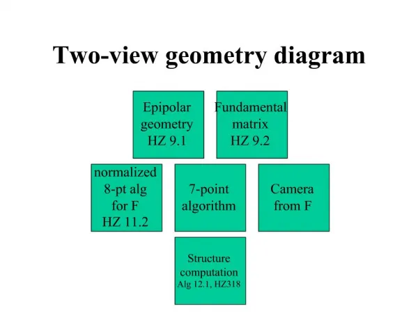
Two-view geometry diagram. Epipolar geometry HZ 9.1. Fundamental matrix HZ 9.2. normalized 8-pt alg for F HZ 11.2. 7-point algorithm. Camera from F. Structure computation Alg 12.1, HZ318. Overview of 2-view geometry. entering Part II of Hartley-Zisserman epipolar geometry

E N D
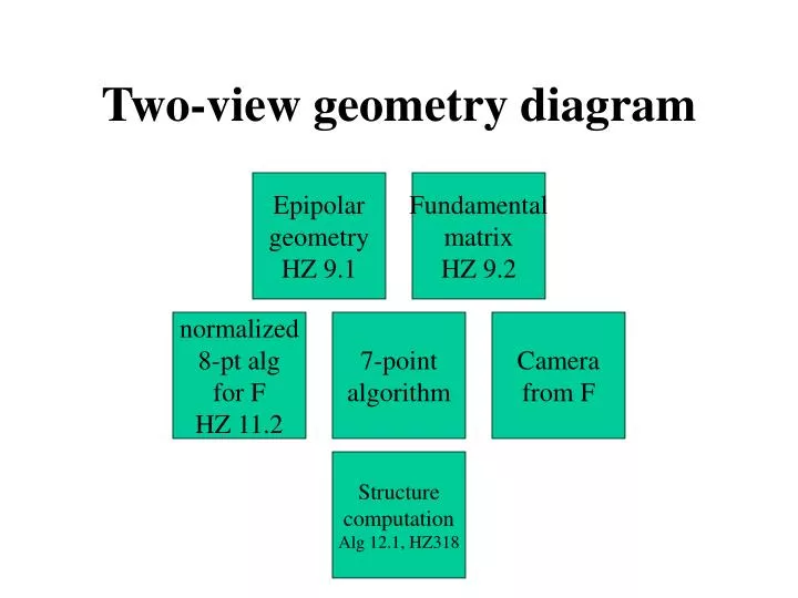
Two-view geometry diagram Epipolar geometry HZ 9.1 Fundamental matrix HZ 9.2 normalized 8-pt alg for F HZ 11.2 7-point algorithm Camera from F Structure computation Alg 12.1, HZ318
Overview of 2-view geometry • entering Part II of Hartley-Zisserman • epipolar geometry • formalization of the structure between 2 views • used to extract depth information inherent in this stereo view • how fundamental matrix F encodes epipolar geometry • the central structure in 2-view geometry is the fundamental matrix F: all of the camera and structure information is extracted directly or indirectly from F • solving for F using point correspondences • 8 point algorithm • singularity constraint • normalization • 7 point algorithm • how the fundamental matrix encodes the camera center and other camera information
Two-view geometry diagram Epipolar geometry HZ 9.1 Fundamental matrix HZ 9.2 normalized 8-pt alg for F HZ 11.2 7-point algorithm Camera from F Structure computation Alg 12.1, HZ318
Finding structure • imagine two cameras (perhaps virtually by moving a single camera in time) • camera centers c and c’ • valid point correspondence (x,x’) • we want to discover the 3D point X associated with this point correspondence • finding X and finding c/c’ are the main goals of structure from motion • we shall explore the geometric relationship between c,c’,x,x’,X
Epipolar geometry • baseline = line cc’ between camera centers; demo: cardboard, 2 frames • epipolar plane = any plane through the baseline • a pencil of planes • epipole = intersection of baseline with image plane • equivalently, image of other camera center • this connection to camera center will be leveraged • crucial to computing structure and camera • note: may lie outside image • epipolar line = intersection of an epipolar plane with an image plane • note: x has an associated epipolar plane (3 points define a plane), so an associated epipolar line • note: x’ lies on the epipolar line associated with x • HZ239-241
Epipolar lines • we have seen that x’ lies on the x epipolar line, and x lies on the x’ epipolar line • offers a mechanism to tie the two points together: if we can compute the epipolar line l’ associated with a point x, then we have a constraint on the position of x’ • l’ . x’ = 0 (x’ lies on l’) • this tells us something about the companion x’ • the fundamental matrix will build epipolar lines from points • so it is valuable in determining structure • epipolar line = image of cx line
Epipoles from epipolar lines • epipolar lines are tied up with epipoles: epipole lies on every epipolar line • notice how the epipole can be found from these epipolar lines • this gives information about the other camera center
Fundamental matrix • the fundamental matrix relates two images • the fundamental matrix F of two images is a 3x3 matrix such that: • F: points epipolar lines • Fx is the epipolar line (in image 2) associated with the point x (in image 1) • also vice versa using Ft: x’ in image 2 => Ft x’ in image 1 • how do we interpret this? x is in a 2-space, Fx is in another 2-space • corollary: xtFx’ = 0 if (x,x’) are a corresponding pair (i.e., image points of the same 3D point X) • proof: x lies on Fx’ • F as epipolar line generator • F as correspondence checker • HZ242
Computing F: basics • we will use xtFx’ = 0 constraints from a few point correspondences to solve for F • each point pair (x,x’) defines a linear equation in F • 8 pairs should be enough to solve for the 8 degrees of freedom in F (projective 3x3) • SIFT will be used to gather point correspondences • detailed algorithms below
Epipoles from F • F yields information about the epipoles (on top of information about epipolar lines and point correspondences) • let e = epipole of image 1 • e’ = epipole of image 2 • both are found as null spaces • Fe = 0 • Ft e’ = 0 • proof below
Interpretation of F • consider the epipolar line l’ associated with x • l’ = e’ x x’ • e’ and x’ lie on l’ • so l’ = [e’]x x’ • skew-symmetric rep • but x’ = Hx for some homography H • can be understood as point transfer off a plane, but not necessary • so l’ = [e’]x Hx • we know l’ = Fx, so: • F = [e’]x H • HZ243
Resulting properties of F • F is rank 2 • [e’]x is rank 2, H is rank 3 • that is, F is singular and has 1d null space • adds a constraint that is very helpful in guiding the computation of F (see below) • proof that Fe = 0: • Fe = ([e’]x H) e = [e’]x (H e) = e’ x (He) = e’ x e’ = 0 • image of e is e’ • thus, the epipole e may be found as the null space of F
CLAPACK • OpenCV has SVD too • www.netlib.org/clapack/ • download CLAPACK from www.netlib.org/clapack/clapack.tgz and www.netlib.org/clapack/clapack.h • install CLAPACK following www.netlib.org/clapack/readme.install • generates lapack_LINUX.a and blas_LINUX.a • optimize the BLAS for your machine (optional) • see my Makefile • see www.netlib.org/lapack for documentation • download the manual pages for ready access: e.g., once you discover through the search engine that ‘sgesv’ solves Ax=b for you, ‘man sgesv’ gives its parameters. • read CLAPACK/readme for caveats of style differences in calling LAPACK from C, such as column-major simulation and call by reference parameters. • sgesvd for SVD