Download
1 / 50
510 likes | 664 Views
A Brief Introduction to Quantum Computation 1 Melanie Mitchell Portland State University. 1 This talk is based on the following paper: E. Rieffel & W. Polak, An introduction to Quantum Computing for Non-Physicists. ACM Computing Surveys , 32(3) 300-335, 2000.

E N D
A Brief Introduction to Quantum Computation1Melanie MitchellPortland State University 1This talk is based on the following paper: E. Rieffel & W. Polak, An introduction to Quantum Computing for Non-Physicists. ACM Computing Surveys, 32(3) 300-335, 2000.
History of Quantum Computation 1982: Richard Feynman, “Simulating physics with computers” • Notes that simulating quantum systems with classical computers is exponential in the number n of particles in the system • Suggests that quantum effects could themselves be used to make such simulations polynomial in n • General idea: due to “superposition” and “entanglement”, state space encoded by quantum system of n particles is exponentially larger than state space encoded by classical system of n particles.
Could this exponential increase in state space be harnessed to create exponential parallelism (2n) with n computing elements? • At that time, no one had any workable ideas about how to build a computer that exploits quantum mechanics. • Also, no one had a detailed model of what a quantum computer would be like. • Also, no one had any algorithms for actually computing anything on a quantum computer.
1985: David Deutsch, “Quantum theory, the Church-Turing principle and the universal quantum computer” • Developed the notion of a universal quantum computer • Gave a simple example of a quantum algorithm that is faster than any known classical algorithm for the same problem
1994, Peter Shor, “Polynomial time algorithms for prime factorization and discrete logarithms on a quantum computer” • Gave quantum algorithm for factoring large numbers in polynomial time, and for performing discrete logs • First major algorithmic result in field of quantum computation • Got a lot of people interested in the field • DARPA, NSF, others started throwing money at it
Other results: • Cryptography: Secure private key communication using qubits. • Grover’s search algorithm: Searches an unstructured list of n items in O(sqrt(n)) on a quantum computer. Known algorithms for classical computers are no better than O(n). • Theory of quantum error correction “It is as yet unknown whether the power of quantum parallelism can be harnessed for a wide variety of applications.” Open question: Can any NP-complete problem be solved in polynomial time on a quantum computer?
Polarization experiment • Polarization of light: electric field vector is confined to a single direction. This is a quantum-mechanical property of photons. • Light source: Assume each photon has a random polarization • Filter A: Horizontally polarized A all photons horizontally polarized photons randomly polarized 1/2 original intensity
Polarization experiment • Polarization of light: electric field vector is confined to a single direction. This is a quantum-mechanical property of photons. • Light source: Assume each photon has a random polarization • Filter A: Horizontally polarized • Filter B: Vertically polarized A B all photons horizontally polarized photons randomly polarized no light
Polarization experiment • Polarization of light: electric field vector is confined to a single direction. This is a quantum-mechanical property of photons. • Light source: Assume each photon has a random polarization • Filter A: Horizontally polarized • Filter B: Vertically polarized • Filter C: polarized at 45 degrees A C B photons randomly polarized 1/8 original intensity
Polarization experiment explanation • Photon’s polarization state can be modeled by a unit vector pointing in the appropriate direction • Let the basis vectors be and • Any polarization can be expressed as where a and b are complex numbers such that
Measurement postulate of quantum mechanics • Any device measuring a quantum system has an associated orthonormal basis with respect to which the measurement takes place. • Measurement of a state transforms the state into one of these basis vectors. • The probability that the state is measured as basis vector u is the norm of the amplitude of the component of the original state in the direction of u.
Example: Let be the polarization state of a photon. Then this state will be measured as with probability |a|2 and as with probability |b|2 . These are indeed probabilities, since . The measurement will also change the state to the result of the measurement. Its original value cannot be determined.
Back to the polarization experiment: • Original light source produces photons with random polarizations: • Thus 50% are measured as horizontal, and let through. (Why?) • Those photons are now in the horizontal state, None are let through by the vertical filter.
Now let the 45o filter be put behind the horizontal filter. The 45o filter measures photon polarization with respect to a new basis: • Photons in state will be measured as with probability 1/2. So half will get through. • Likewise, filter B will let half of these through. • Total photons getting through all three filters: (1/2)3 = 1/8.
Bra/Ket notation Ket: • Column vector, used to describe quantum states • E.g., can be written as • In general, Bra: • Conjugate transpose of
Quantum bits (“qubits”) A qubit is a unit vector in a two-dimensional complex vector space. Assume a particular basis, denoted by These basis states represent the classical bit values 0 and 1. However, unlike classical bits, qubits can be in a superposition of these two states, e.g., such that
Suppose a qubit (a, b)T is measured with respect to the basis Probability that will be measured is |a|2, and Probability that will be measured is |b|2. When a qubit is measured, its state becomes the basis state that was measured. All information about the original superposition is lost.
Example of using qubits: Quantum key distribution(Bennett & Brassard, 1987) • Solves problem of secure key distribution for private key cryptography • Public key cryptography using RSA is great, but relies on factoring being a hard problem. • Private key cryptography is in principle more secure, but relies on private key being securely transmitted. • Quantum method gives perfect security in private key transmission
= 0 = 1 = 0 = 1 1 1 0 1 1 1 0 0 0 0 Alice wants to send a key to Bob by encoding each bit as the quantum state of a photon. She secretly encodes each bit by randomly choosing one of two basis: or E.g.,
What Alice sent 1 1 0 1 1 1 0 0 0 0 What Bob measured Basis: ud diag ud diag ud ud diag ud diag diag Measurement: 1 0 0 1 1 1 1 0 1 0 Bob measures the state of each photon he receives by randomly picking either basis, up-down (ud), or diagonal (diag). Now Alice and Bob communicate what bases they used for each measurement. They save only the bits for which they used the same bases (approx. 50%). These bits form the private key.
What Alice sent 1 1 0 1 1 1 0 0 0 0 What Bob measured Basis: ud diag ud diag ud ud diag ud diag diag Measurement: 1 0 0 1 1 1 1 0 1 0 Bob measures the state of each photon he receives by randomly picking either basis, up-down (ud), or diagonal (diag). Now Alice and Bob communicate what bases they used for each measurement. They save only the bits for which they used the same bases (approx. 50%). These bits form the private key.
Now, suppose a third person, Eve, intercepts the stream of photons from Alice, measures their states, and sends new photons with the measured states to Bob. She will choose the wrong basis 50% of the time. So on the photons for which Bob chooses the same basis as Alice, 25% of them will be incorrect. Bob and Alice can detect this error by sending sample “correct” (parity) bits to each other over open communication line. Thus they can detect an eavesdropper.
Multiple qubits • Suppose you have n particles whose states are each vectors in a 2-D vector space (e.g., x, y position) • How many dimensions do you need to describe complete state of the system? • Particles have coordinates (x1, y1), (x2, y2), ..., (xn, yn) • Complete state is simply a list of all the coordinates: (x1, y1, x2, y2, ..., xn, yn) • I.e., 2n dimensions
Quantum case is different due to “entanglement”. • Again, suppose you have n particles whose states are each vectors in a 2-D vector space. • Particles have coordinates (x1, y1), (x2, y2), ..., (xn, yn) • Complete state is more complicated, due to entanglement of states: (x1x2x3...xn-1xn, x1x2x3...xn-1yn, x1x2x3...yn-1xn, ...) • I.e., 2ndimensions
y (1, 2) (2, 1) x Example: n = 2 • Classical basis vectors: (1, 0), (0, 1) • Classical state of system: ( (1, 2), (2, 1) ) • Quantum basis vectors: (1, 0) (1,0) = (1, 0, 0, 0) (1, 0) (0,1) = (0, 0, 1, 0) (0, 1) (1,0) = (0, 1, 0, 0) (0, 1) (0, 1)= (0, 0, 0, 1) • Quantum state of system: Linear combination of those basis vectors
y (1, 2) (2, 1) x Interpretation: In quantum system you now need four numbers to give the state of the two-particle system. Each dimension describes a particular entanglement of the original dimensions of the individual particles.
In quantum computation, the “particles” are the qubits. Each qubit has a state defined by two complex numbers: A two-qubit state is defined by four complex numbers:
Recall the notion of superposition: • A single qubit is in a superposition of two basis states: • A 3-qubit system is in a superposition of eight basis states: where a1, a2, ..., an are complex numbers such that • In general, an n-qubit system is in a superposition of 2n basis states.
This exponential increase in size of state space as n increases is why classical computers cannot efficiently simulate quantum systems. • This was Feynman’s impetus for proposing quantum computers.
Measurement in entangled systems • Example 1: The state is entangled: • If no bits have yet been measured, the probability of measuring the first (or second) bit as is 0.5. • However, if the second (or first) bit has been measured, the probability is 0 or 1, depending on what the second (or first) bit was measured to be.
Example 2: The state is not entangled: Can factor out first bit: it will always be measured as . Measuring it does not affect the second bit.
EPR paradox(Einstein, Podolsky, Rosen, “Can quantum-mechanical description of physical reality be considered complete?” (1935)) • Imagine a source that generates two maximally entangled particles: • One particle is sent to Alice, and the other to Bob. • Suppose Alice measures her particle and observes state . • Then the combined state will now be . This means Bob will also measure . • The change in state occurs instantaneously, no matter how far away Alice and Bob are from each other.
Does this allow communication faster than the speed of light? • EPR’s explanation: • Each particle has a “hidden” internal state that determines what the result of any given measurement will be. • Called “local hidden variable theory”. • Einstein: “God does not play dice.” • Problem with this explanation: • Doesn’t explain measurements with respect to a different basis. • Bell’s theorem: predicts an inequality that must be satisfied if hidden variable theory is correct. • Experiments show it to be incorrect.
Cause and effect explanation: • Somehow Alice’s measurement causes the result found by Bob, • Problems with this explanation: • Violates relativity theory: Can set up experiment where one observer sees Alice do measurement first, while other observer sees Bob do measurement first. This does not change the results of the measurements. • This also shows that Alice and Bob can’t use their particles to communicate faster than the speed of light. • “All that can be said is that Alice and Bob will observe the same random behavior.”
From Black et al., “Quantum computing and communications” (2002): “The ugly truth is that general relativity and quantum mechanics are not consistent. That is, our current formulations of general relativity and quantum mechanics give different predictions for extreme cases. We assume there is a ‘Theory of Everything’ that reconciles the two, but it is still very much an area of thought and research. Since relatively is not needed in quantum computing, we ignore this problem.”
Hadamard transformation How are I, X, Y, Z, and H implemented in a physical quantum computer? That’s beyond the scope of this talk....
Walsh-Hardamard Transformation For example:
Quantum Gate Arrays • Uf is a quantum gate array that implements function f (Deutsch proved Uf can be constructed for any computable function f) • To compute f(x), apply Uf to tensored with a “register” of :
Quantum Parallelism • To get exponential parallelism, apply Uf to an input that is in a superposition of all inputs. • Result will be superposition of all results of applying f(x) to all inputs. • Quantum algorithm to compute function f(x): • Start with n-qubit state
Apply Walsh-Hadamard transformation W to this state to get a superposition of all integers in [0, 2n-1]:
Tensor this state with a “register” of one or more zero qubits: • Now apply Ufto this state: • Result is superposition of f(x) for all integers x[0,2n-1] • This is what is meant by quantum parallelism.
Example: Consider quantum AND gate (“Toffoli gate”): • Now prepare superposition of all possible bit combinations of x and y, together with the “register” :
Now, apply T to this superposition: • The resulting quantum state, obtained in one step, gives a superposition of all possible results for the AND function for two bits. • What happens if we measure this quantum state? • Need clever techniques to allow user to read out a desired result.
Photo gallery Peter Shor Edward Fredkin Tomosso Toffoli David Deutsch Richard Jozsa
Very brief outline of Shor’s algorithm for factoring We have a composite number M, and we want to find a factor of M. Approach: Reduce the problem of factoring to the problem of finding the period of an integer function, f(x)=ax (mod M), for some a. Problem there is no known classical polynomial time algorithm to find period r.
Guess integers a and m (with some constraints). Define f(x) = ax (mod M). • Create a quantum state of m zero qubits along with a extra register of qubits: Apply the Walsh-Hadamard transform to obtain an equal-probability superposition of all integers from 0 to 2m-1:
Now use Uf to compute f (x) for all integers from 0 to 2m-1 simultaneously: • From this state, create a new (related) state whose amplitude has the same period as f. To do this, measure the qubits that encode f(x). Suppose it is measured as u.
Actually, we don’t care about u; we only care about the side effect of measurement: the quantum state is now where C is a scale factor, and Note that the period of g(x) equals the period of f (x). If we could measure two successive x’s in the sum, we would know the period. But we can only do one measurement.
Take the quantum Fourier transform of this new state. • Extract the period r. If period is a power of 2, this can be done exactly. If not, “guess” the period, using “continued fractions”. • Now can apply Euclid’s algorithm (polynomial time) to obtain a factor of M from the period r. If it fails, start over with a new guess for a and m. Shor showed that this algorithm has high probability of succeeding after only a few repetitions.