Download
1 / 48
710 likes | 1.65k Views
The Standard Regression Model and its Spatial Alternatives. Relationships Between Variables and Building Predictive Models . . Spatial Statistics. . Descriptive Spatial Statistics: Centrographic Statistics single, summary measures of a spatial distribution

E N D
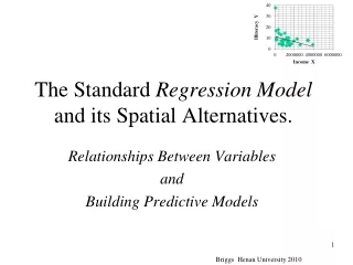
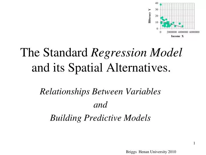
The Standard Regression Model and its Spatial Alternatives. Relationships Between Variables and Building Predictive Models Briggs Henan University 2010
Spatial Statistics Descriptive Spatial Statistics: Centrographic Statistics single, summary measures of a spatial distribution - Spatial equivalents of mean, standard deviation, etc.. Inferential Spatial Statistics: Point Pattern Analysis Analysis of point location only--no quantity or magnitude (no attribute variable) --Quadrat Analysis --Nearest Neighbor Analysis, Ripley’s K function Spatial Autocorrelation One attribute variable with different magnitudes at each location The Weights Matrix Global Measures of Spatial Autocorrelation (Moran’s I, Geary’s C, Getis/Ord Global G) Local Measures of Spatial Autocorrelation (LISA and others) Prediction with Correlation and Regression Two or more attribute variables Standard statistical models Spatial statistical models Briggs Henan University 2010
Bivariate and Multivariate income education Y income gender* education X1 X2 *Gender = male or female Briggs Henan University 2010 • All measures so far have focused on one variable at a time • univariate • Often, we are interested in the association or relationship between two variables • bivariate. • Or more than two variables • multivariate
Correlation and RegressionThe most commonly used techniques in science. Review standard (non-spatial) approaches Correlation Regression Spatial Regression Why it is necessary. How to do it. Briggs Henan University 2010
Correlation and RegressionWhat is the difference? Regression line predicts Briggs Henan University 2010 • Mathematically, they are identical. • Conceptually, very different. Correlation • Co-variation • Relationship or association • No direction or causation is implied • Y X X1 X2 Regression • Prediction of Y from X • Implies, but does not prove, causation • X (independent variable) Y (dependent variable)
Correlation Coefficient (r) • The most common statistic in all of science • measures the strength of the relationship (or “association”) between two variables e.g. income and education • Varies on a scale from –1 thru 0 to +1 +1 implies a perfect positive association • As values go up () on one, they also go up () on the other • income and education 0 implies no association -1 implies perfect negative association • As values go up on one () , they go down () on the other • price and quantity purchased • Full name is the Pearson Product Moment correlation coefficient, () () () () -1 0 +1 Briggs Henan University 2010
Examples of Scatter Diagrams and the Correlation Coefficient Positive r = 1 r = 0.72 Income perfect positive strong positive Education r = 0.26 Negative weak positive r = -0.71 r = -1 Quantity perfect negative strong negative Price Briggs Henan University 2010
Correlation Coefficient: example Correlation coefficient = 0.9458 (see later for calculation) China Provinces 29 excludes Xizang/Tibet, Macao, Hong Kong, Hainan, Taiwan, P'eng-hu Briggs Henan University 2010
å n 2 ( Y Y ) Sy= - i n - - å ( x X )( y Y ) = 1 i i i = N = i 1 r n S S å n 2 ( X X ) x y SX= - i = i 1 N Pearson Product Moment Correlation Coefficient (r) Moments about the mean “product” is the result of a multiplication X * Y = P Where Sx and Sy are the standard deviations of X and Y, and X and Y are the means. Briggs Henan University 2010
Calculation Formulae for Correlation Coefficient (r) Before the days of computers, these formulae where easier to do “by hand.” See next slide for example Briggs UT-Dallas GISC 6382 Spring 2007
Correlation Coefficient example using “calculation formulae” Scatter Diagram Source: Lee and Wong Briggs Henan University 2010
Regression Y X Y income gender* education X1 X2 Briggs Henan University 2010 • Simple regression • Between two variables • One dependent variable (Y) • One independent variable (X) • Multiple Regression • Between three or more variables • One dependent variable (Y) • Two or independent variable (X1 ,X2…)
Y b 1 a X Simple Linear Regression • Concerned with “predicting” one variable (Y - the dependent variable) from another variable (X - the independent variable) Y = a +bX + = residual= error = Yi-Ŷi =Actual (Yi ) – Predicted (Ŷi) • a is the intercept —the value of Y when X =0 • b is the regression coefficient or slope of the line • —the change in Y for a one unit change in X Yi Regression line Ŷi X 0 Briggs Henan University 2010
Ordinary Least Squares (OLS)--the standard criteria for obtaining the regression line The regression line minimizes the sum of the squared deviations between actual Yi and predicted Ŷi Yi Ŷi Min (Yi-Ŷi)2 Yi Ŷi Briggs Henan University 2010
Coefficient of Determination (r2) SS Regression or Explained Sum of Squares SS Total or Total Sum of Squares Note: SS Residual or Error Sum of Squares SS Total or Total Sum of Squares SS Regression or Explained Sum of Squares + = • The coefficient of determination (r2) measures the proportion of the variance in Y (the dependent variable) which can be predicted or “explained by” X (the independent variable). Varies from 1 to 0. • It equals the correlation coefficient (r) squared.
Partitioning the Variance on Y Y Y Y SS Residual or Error Sum of Squares SS Total or Total Sum of Squares SS Regression or Explained Sum of Squares Briggs Henan University 2010
Standard Error of the Estimate (se) Sum of squared residuals Number of observations minus degrees of freedom (for simple regression, degrees of freedom = 2) Briggs Henan University 2010 Measures predictive accuracy: the bigger the standard error, the greater the spread of the observations about the regression line, thus the predictions are less accurate Se2= error mean square, or average squared residual = variance of the estimate, variance about regression (called sigma-square in GeoDA)
Coefficient of determination (r2 ), correlation coefficinet (r), regression coefficient (b), and standard error (Se) (Values are hypothetical and for illustration of relative change only) r2 = 0.94 r = .97 Se= 0.3 r2 = r = 1 Se= 0.0 Sy = 2 b = 2 r2 = 0.51 r = .71 Se= 1.1 b = 1.1 perfect positive Very strong strong r2 = 0.26 r = .51 Se= 1.3 b = 0.8 r2 = 0.07 Se= 1.8 b = 0.1 r2 = r= 0.00 Se= Sy = 2 moderate weak none b = 0 As the coefficient of determination gets smaller, the slope of the regression line (b) gets closer to zero. As the coefficient of determination gets smaller, the standard error gets larger, and closer to the standard deviation of the dependent variable (Y) (Sy = 2) Regression line in blue
Sample Statistics, Population Parameters and Statistical Significance tests Briggs Henan University 2010 Yi = a +bXi +ia and b are sample statistics which are estimates of population parametersα and β β (and b) measure the change in Y for a one unit change in X. If β = 0 then X has no effect on Y, therefore Null Hypothesis (H0): in the population β = 0 Alternative Hypothesis (H1): in the population β ≠ 0 Thus, we test if our sample regression coefficient, b, is sufficiently different from zero to reject the Null Hypothesis and conclude that X has a statistically significant affect on Y
Test Statistics in Simple Regression Briggs Henan University 2010 Test statistic for b is distributed according to the Student’s t Distribution (similar to normal): where is the variance of the estimate, with degrees of freedom = n – 2 A test can also be conducted on the coefficient of determination (r2 ) to test if it is significantly greater than zero, using the F frequency distribution. It is mathematically identical to the t test.
Multiple regression We can rewrite simple regression as: Multiple regression: Y is predicted from 2 or more independent variables • β0is the intercept —the value of Y when values of all Xj = 0 • β1… β m are partialregression coefficients which give the change in Y for a one unit change in Xj, all other X variables held constant • m is the number of independent variables Y income gender* education X1 X2 Briggs Henan University 2010
Multiple regression: least squares criteria or As in simple regression, the “least squares” criteria is used. Regression coefficients bj are chosen to minimize the sum of the squared residuals (the deviations between actual Yi and predicted Ŷi) The difference is that Ŷi is predicted from 2 or more independent variables, not one. Regression hyperplane
Coefficient of Multiple Determination (R2) SS Regression or Explained Sum of Squares SS Total or Total Sum of Squares Formulae identical to simple regression As with simple regression SS Residual or Error Sum of Squares SS Total or Total Sum of Squares SS Regression or Explained Sum of Squares + = • Similar to simple regression, the coefficient of multiple determination (R2) measures the proportion of the variance in Y (the dependent variable) which can be predicted or “explained by” all of X variables in combination. Varies from 0 to 1.
Reduced or Adjusted Not perfect perfect Y k is the number of coefficients in the regression equation, normally equal to the number of independent variables plus 1 for the intercept. X1 X2 Briggs Henan University 2010 • R2 will always increase each time another independent variable is included • an additional dimension is available for fitting the regression hyperplane (the multiple regression equivalent of the regression line) • Adjusted is normally used instead of R2 in multiple regression
Y b 1 a X Interpreting partial regression coefficients • The regression coefficients (bj) tell us the change in Y for a 1 unit change in Xj, all other X variables “held constant” • Can we compare these bj values to tell us the relative importance of the independent variables in affecting the dependent variable? • If b1 = 2 and b2 = 4, is the affect of X2 twice as big as the affect of X1 ? • No, no, no in general!!!! • The size of bj depends on the measurement scale used for each independent variable • if X1 is income, then a 1 unit change is $1 • but if X2 is rmb or Euro(€) or even cents (₵) 1 unit is not the same! • And if X2 is % population urban, 1 unit is very different • Regression coefficients are only directly comparable if the units are all the same: all $ for example
Standardized partial regression coefficientsComparing the Importance of Independent Variables Note the confusing use of β for both standardized partial regression coefficients and for the population parameter they estimate. • How do we compare the relative importance of independent variables? • We know we cannot use partial regression coefficients to directly compare independent variables unless they are all measured on the same scale • However, we can use standardized partial regression coefficients (also called beta weights, beta coefficients, or path coefficients). • They tell us the number of standard deviation (SD) unit changes in Y for a one SD change in X) • They are the partial regression coefficients if we had measured every variable in standardized form
Test Statistics in Multiple Regression:testing each independent variable with degrees of freedom = n – k, where k is the number of coefficients in the regression equation, normally equal to the number of independent variables plus 1 for the intercept (m+1). The formula for calculating the standard error (SE) of bj is more complex than for simple regression , so it is not shown here. Briggs Henan University 2010 A test can be conducted for each partial regression coefficient bj to test if the associated independent variable influences the dependent variable. It is distributed according to the Student’s t Distribution (similar to the normal frequency distribution): Null Hypothesis Ho : bj = 0 .
Test Statistics in Mutiple Regressiontesting the overall model Again, k is the number of coefficients in the regression equation, normally equal to the number of variables (m) plus 1. • We test the coefficient of multiple determination (R2 ) to see if it is significantly greater than zero, using the F frequency distribution. • It is an overall test to see if at least one independent variable, or two or more in combination, affect the dependent variable. • Does not test if each and every independent variable has an effect • Similar to the F test in simple regression. • But unlike simple regression, it is not identical to the t tests. • It is possible (but unusual) for the F test to be significant but all t tests not significant.
Always look at your data Don’t just rely on the statistics! Anscombe's quartet Summary statistics are the same for all four data sets: mean (7.5), standard deviation (4.12), correlation (0.816) regression line (y = 3 + 0.5x). Anscombe, Francis J. (1973). "Graphs in statistical analysis". The American Statistician27: 17–21. Briggs Henan University 2010
Real data is almost always more complex than the simple, straight line relationship assumed in regression. Waiting time between eruptions and the duration of the eruption for the Old Faithful Geyser in Yellowstone National Park, Wyoming, USA. This chart suggests there are generally two "types" of eruptions: short-wait-short-duration, and long-wait-long-duration. Source: Wikipedia Briggs Henan University 2010
Spurious relationships Eating ice cream inhibits swimming ability. --eat too much, you cannot swim Omitted variable problem --both are related to a third variable not included in the analysis Help! Summer temperatures: --more people swim (and some drown) --more ice cream is sold Briggs Henan University 2010
Regression does not prove direction or cause!Income and Illiteracy Illiteracy Income Income Illiteracy Briggs Henan University 2010 • Provinces with higher incomes can afford to spend more on education, so illiteracy is lower • Higher Income>>>>Less Illiteracy • The higher the level of literacy (and thus the lower the level of illiteracy) the more high income jobs. • Less Illiteracy>>>>Higher Income • Regression will not decide!
Spatial Regression It doesn’t solve any of the problems just discussed! You always must examine your data! Briggs Henan University 2010
Spatial Autocorrelation & Correlation Spatial Autocorrelation: shows the association or relationship between the same variable in “near-by” areas. Standard Correlation shows the association or relationship between two different variables Each point is a geographic location Education “next door” income In a neighboring or near-by area education education Briggs Henan University 2010
If Spatial Autocorrelation exists: • correlation coefficients and coefficients of determination appear bigger than they really are • biased upward • You think the relationship is stronger than it really is • the variables in nearby areas affect each other • Standard errors appear smaller than they really are • exaggerated precision • You think your predictions are better than they really are since standard errors measure predictive accuracy • More likely to conclude relationship is statistically significant. (We discussed this in detail in the lecture on Spatial Autocorrelation concepts.) Briggs Henan University 2010
How do I know if I have a problem? Briggs Henan University 2010 For correlation, calculate Moran’s I for each variable and test its statistical significance • If Moran’s I is significant, you may have a problem! For regression, calculate the residuals Yi-Ŷi =Actual (Yi ) – Predicted (Ŷi) Then: • map the residuals: do you see any spatial patterns? --if yes, you may have a problem • Calculate Moran’s I for the residuals: is it statistically significant? --if yes, you have a problem
What do I do if SA exists? Briggs Henan University 2010 Acknowledge in your paper that SA exists and that the calculated correlation coefficients may be larger than their true value, and may not be statistically significant Try to fix the problem!
How do I fix SA? Briggs Henan University 2010 Step 1: Try to identify omitted variables and include them in a multiple regression. • Missing (omitted) variables may cause spatial autocorrelation • Regression assumes all relevant variables influencing the dependent variable are included • If relevant variables are missing, model is misspecified Step 2: If additional variables cannot be identified, or SA still exists, use a spatial regression model
Spatial Regression: 4 Options • Getis, A. and Daniel Griffith (2002) Comparative Spatial Filtering in Regression AnalysisGeographical Analysis 34 (2) 130-140 • Spatial Autoregressive Models • Lag model • Error model • Spatial Filtering --based on eigenfunctions (Griffith) • Spatial Filtering --based on Ripley’s K and Getis-Ord G (Getis) • Others We will consider the first option only. • simpler and the more commonly used • Getis and Griffith 2002 compare the first three
Spatial Lag and Spatial Error Models:mathematical comparison • Spatial lag model • values of the dependent variable in neighboring locations (WY) are included as an extra explanatory variable • these are the “spatial lag” of Y • Spatial error model • values of the residuals in neighboring locations (Wε) are included as an extra term in the equation; • these are “spatial error” • W is the spatial weights matrix Y = β0 + λWY + Xβ + ε Y = β0 + Xβ + ρWε+ ξ ξ is “white noise”
Spatial Lag and Spatial Error Models:conceptual comparison Ordinary Least Squares OLS SPATIAL LAG SPATIAL ERROR Dependent variable influenced by neighbors No influence from neighbors Residuals influenced by neighbors Baller, R., L. Anselin, S. Messner, G. Deane and D. Hawkins. 2001. Structural covariates of US County homicide rates: incorporating spatial effects,. Criminology , 39, 561-590 Briggs Henan University 2010
Lag or Error Model: Which to use? Briggs Henan University 2010 • Lag model primarily controls spatial autocorrelation in the dependent variable • Error model controls spatial autocorrelation in the residuals, thus it controls autocorrelation in both the dependent and the independent variables • Conclusion: the error model is more robust and generally the better choice. • Statistical tests called the LM Robust test can also be used to select • Will not discuss these
Comparing our models k is the number of coefficients in the regression equation, normally equal to the number of independent variables plus 1 for the intercept term. Akaike, Hirotuga (1974) A new look at statistical model identification IEEE Transactions on Automatic Control 19 (6) 716-723 Briggs Henan University 2010 • Which model best predicts the dependent variable? • Neither R2 nor Adjusted can be used to compare different spatial regression models • Instead, we use Akaike Information Criteria (AIC) • the smaller the AIC value the better the model Note: can only be used to compare models with the same dependent variable
Geographically Weighted Regression • The idea of Local Indicators can also be applied to regression • Its called geographically weighted regression • It calculates a separate regression for each polygon and its neighbors, • then maps the parameters from the model, such as the regression coefficient (b) and/or its significance value • Mathematically, this is done by applying the spatial weights matrix (Wij) to the standard formulae for regression See Fotheringham, Brunsdon and Charlton Geographically Weighted Regression Wiley, 2002 Xi Briggs Henan University 2010
Problems with Geographically Weighted Regression Xi Briggs Henan University 2010 • Each regression is based on few observations • the estimates of the regression parameters (b) are unreliable • Need to use more observations than just those with shared border, but • how far out do we go? • How far out is the “local effect”? • Need strong theory to explain why the regression parameters are different at different places • Serious questions about validity of statistical inference tests since observations not independent
What have we learned today? Briggs Henan University 2010 • Correlation and regression are very good tools for science. • Spatial data can cause problems with standard correlation and regression • The problems are caused by spatial autocorrelation • We need to use Spatial Regression Models • Geographers and GIS specialists are experts on spatial data • They need to understand these issues!