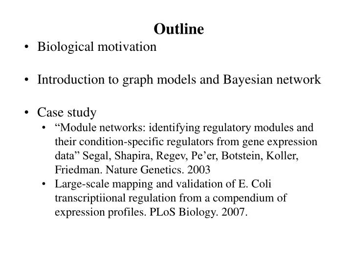
Outline Biological motivation Introduction to graph models and Bayesian network Case study

1. Outline • Biological motivation • Introduction to graph models and Bayesian network • Case study • “Module networks: identifying regulatory modules and their condition-specific regulators from gene expression data” Segal, Shapira, Regev, Pe’er, Botstein, Koller, Friedman. Nature Genetics. 2003 • Large-scale mapping and validation of E. Coli transcriptiional regulation from a compendium of expression profiles. PLoS Biology. 2007.

2. 1. Biological motivation • cis-regulatory motif: A short (6-to-12-ish) series of DNA bases that can bind to an “activator” or “repressor” protein. Illustrated at right as activator/repressor binding sites.

3. 1. Biological motivation • Module: set of genes that participate in a coherent biological process • Module group: set of modules that all share at least one cis-regulatory motif • regulator: a gene that encodes a protein whose concentration regulates the expression of other genes • expression profile: concentrations of various genes in given bio-experimental circumstances

4. 1. Biological motivation

5. 2. Introduction to Bayesian Network "Graphical models are a marriage between probability theory and graph theory. They provide a natural tool for dealing with two problems that occur throughout applied mathematics and engineering -- uncertainty and complexity. ……..Fundamental to the idea of a graphical model is the notion of modularity -- a complex system is built by combining simpler parts. Probability theory provides the glue whereby the parts are combined, ensuring that the system as a whole is consistent. Many of the classical multivariate probabalistic systems are special cases of the general graphical model formalism -- examples include mixture models, factor analysis, hidden Markov models, Kalman filters and Ising models.…..the graphical model formalism provides a natural framework for the design of new systems." --- Michael Jordan, 1998.

6. 2. Introduction to Bayesian Network P(C)=0.5, P(-C)=0.5 Cloudy Sprinkler Rain P(S|C)=0.1, P(-S|C)=0.9 P(S|-C)=0.5, P(-S|-C)=0.5 P(R|C)=0.8, P(-R|C)=0.2 P(R|-C)=0.2, P(-R|-C)=0.8 Wet Grass P(W|S,R)=0.99, P(-W|S,R)=0.01 P(W|S,-R)=0.9, P(-W|S,-R)=0.1 P(W|-S,R)=0.9, P(-W|-S,R)=0.1 P(W|-S,-R)=0, P(-W|-S,-R)=1 From: http://www.cs.ubc.ca/~murphyk/Bayes/bnintro.html

7. 2. Introduction to Bayesian Network • Graphs in which nodes represent random variables (cloudy? sprinkler? rain? wet grass) • Arrows represent conditional independence assumptions. (e.g. P(W|S,R,C)=P(W|S,R)) • Present & absent arrows provide compact representation of joint probability distributions • BNs have complicated notion of independence, which takes into account the “directionality” of the arrows

8. 2. Introduction to Bayesian Network Bayes’ Rule Can rearrange the conditional probability formula to get P(A|B) P(B) = P(A,B), but by symmetry we can also get: P(B|A) P(A) = P(A,B) It follows that:  The power of Bayes' rule is that in many situations where we want to compute P(A|B) it turns out that it is difficult to do so directly, yet we might have direct information about P(B|A). Bayes' rule enables us to compute P(A|B) in terms of P(B|A).

9. 2. Introduction to Bayesian Network Need prior P for root nodes and conditional Ps, that consider all possible values of parent nodes, for nonroot nodes. Cloudy P(C)=0.5, P(-C)=0.5 Sprinkler Rain P(R|C)=0.8, P(-R|C)=0.2 P(R|-C)=0.2, P(-R|-C)=0.8 P(S|C)=0.1, P(-S|C)=0.9 P(S|-C)=0.5, P(-S|-C)=0.5 Wet Grass P(W|S,R)=0.99, P(-W|S,R)=0.01 P(W|S,-R)=0.9, P(-W|S,-R)=0.1 P(W|-S,R)=0.9, P(-W|-S,R)=0.1 P(W|-S,-R)=0, P(-W|-S,-R)=1 From: http://www.cs.ubc.ca/~murphyk/Bayes/bnintro.html

10. Major benefit of BN 2. Introduction to Bayesian Network • We can know P(W) based only on the conditional probabilities of W and its parent nodes (R and S). We don’t need to know/include all the ancestor probabilities between W and the root nodes (C) . Cloudy Sprinkler Rain Wet Grass

11. 2. Introduction to Bayesian Network This BN benefit hugely reduces # of numbers and computations needed for large networks, e.g. hundreds or thousands of genes • SSR article: many separate Bayesian networks generated based on gene expression data. Here one activator and one repressor form basic BN, with 3 corresponding expression “contexts” shown at bottom.

12. 2. Introduction to Bayesian Network Cloudy P(C)=0.5, P(-C)=0.5 Order of reduction of required numbers:Reduce from 24-1=15 to 9 Sprinkler Rain P(R|C)=0.8, P(-R|C)=0.2 P(R|-C)=0.2, P(-R|-C)=0.8 P(S|C)=0.1, P(-S|C)=0.9 P(S|-C)=0.5, P(-S|-C)=0.5 Wet Grass P(W|S,R)=0.99, P(-W|S,R)=0.01 P(W|S,-R)=0.9, P(-W|S,-R)=0.1 P(W|-S,R)=0.9, P(-W|-S,R)=0.1 P(W|-S,-R)=0, P(-W|-S,-R)=1 From: http://www.cs.ubc.ca/~murphyk/Bayes/bnintro.html

13. 2. Introduction to Bayesian Network Bayesian network: general formulation Given a graph G, the likelihood of observing the data D: De Jong (2002)

14. 2. Introduction to Bayesian Network Evaluating Bayesian networks: • Generally NP hard! Where do the numerical estimates of probability come from? • Can be, at least initialized with, expert opinion • Can be learned by system • Both SSR and BSK articles lay out basics and some details of iterative algorithms for finding probability numbers.

15. 2. Introduction to Bayesian Network Modellinging regulatory network De Jong (2002)

16. 3. Case study • “Module networks: identifying regulatory modules and their condition-specific regulators from gene expression data” Segal, Shapira, Regev, Pe’er, Botstein, Koller, Friedman [SSR] Nature Genetics, June 2003 • Bayesian network-based algorithms are applied to gene expression data to generate good testable hypotheses.

17. 3. Case study • Expression data set, from Patrick Brown’s lab, is for genes of yeast subjected to various kinds of stress • Compiled list of 466 candidate regulators • Applied analysis to 2355 genes in all 173 arrays of yeast data set • This gave automatic inference of 50 modules of genes • All modules were analyzed with external data sources to check functional coherence of gene products and validity of regulatory program • Three novel hypotheses suggested by method were tested in bio lab and found to be accurate

18. 3. Case study

19. 3. Case study

20. 3. Case study • 2 examples of 50 modules inferred by SSR methods: • Respiration – mostly genes encoding respiration proteins or glucose-metabolism proteins. One primary regulator predicted – Hap4 – which is known from past experiments to play activation role in respiration. Secondary regulators affect Hap4 expression. • Nitrogen catabolite repression – 29 genes tied to process by which yeast uses best available nitrogen source. Key regulator suggested is Gat1, due to 26 of 29 genes having Gat1 regulatory motif in their upstream regions.

21. 3. Case study Respiration Network: Two major motifs found

22. 3. Case study • Evaluating module content and regulation programs • All 50 modules were tested to see if proteins coded in same module had related functions • Scored modules on how many genes are noted in current bio databases as being related to the predicted function – diagram, next slide • 31 of 50 modules had coherence >50%; only 4 had coherence <30%.

23. 3. Case study Colored boxes indicate that known experimental evidence validates the predicted regulatory role of a regulator (named in one of the ‘Reg’ columns) in a given module (each row of the table). M, C and G column headers and different colors of boxes represent different sorts of experimental evidence that validate the model’s prediction. C(%): functional coherence of module, from literature mentions of module genes. #G: number of genes in module

24. 3. Case study • To find global relationships between modules, graph (next 2 slides) made showing modules & their motifs. Motifs were found within the 500 base pairs upstream from each gene. • Observations from this graph: modules with related biological functions often shared at least one motif, & sometimes shared one or more regulator genes.

25. 3. Case study Module relationships Yeast mutants of Kin82, Ppt1, Ypl230W were further tests to validate their relationship with the module.

26. 3. Case study

27. 3. Case study What does a BN look like here? • Need to specify two things to describe a BN • Graph topology (structure) • Parameters of each conditional probability distribution • Possible to learn both from data • Learning structure is much harder than learning parameters

28. 3. Case study What can we learn?Why the Segal’s paper can be successful? • Yeast! Not mouse or human. • Use gene clustering first. Start from simplified hypothesis and a small set of known regulators; not to attempt a network of thousands of genes. • Experimental validation.

29. Network measures

30. Networks • Key elements: nodes and edges • Binary network vs weighted network • Directed vs undirected network One simple way to generate a binary gene expression network: • Calculate Pearson or Spearman correlation of each pair of genes. • Use a threshold d (e.g d=0.6) to determine presence of an edge.

31. Connectivity (degree) Degree of node is the number of edges connected to the node. For example: Deg(a)=4 Deg(c)=5

32. Clustering coefficient The (local) clustering coefficient of node i is a density measure of local connections, or “cliquishness”. For example: ClusterCoef(a)=4/6=0.66667 4 triangles involving a: (d,a,b) (c,a,g) (d,a,c) (d,a,g) ClusterCoef(b)=2/6=0.33333

33. Shortest pathlength The shortest path length from one node to another. For example: Shortest path (from a to e): a->d->e, thus of length 2 Shortest path (from a to g); a->g, thus of length 1

34. Betweenness centrality Betweenness centrality is a measure of a node's centrality in a network equal to the number of shortest paths from all vertices to all others that pass through that node. Betweenness centrality is a more useful measure of the load placed on the given node in the network as well as the node's importance to the network than just connectivity. For example: g(c)=2.5 g-e 1/2 f-a 1/3 f-d 1/3 f-e 1 a-e 1/3

35. Network density The network density (also known as line density (Snijders 1981)) is defined as the mean off-diagonal adjacency and is closely related to the mean connectivity. Density In this network: Off diagonal connectivity sum is 14. So the density equals: 14/choose(7,2)=0.66667

36. Assortativity The assortativity coefficient is the Pearson correlation coefficient of degree between pairs of linked nodes. Hence, positive values of r indicate a correlation between nodes of similar degree, while negative values indicate relationships between nodes of different degree. In this network: Assortativity is -0.296

37. Small-world network Small world property: Most nodes are not neighbors of one another, but most nodes can be reached from every other by a small number of hops or steps. Denote by distance L between two randomly chosen nodes (the number of steps required by shortest path) grows proportionally to the logarithm of the number of nodes N in the network, that is: L  log N

38. Scale-free network A scale-free network is a network whose degree distribution follows a power law, at least asymptotically. That is, the fraction P(k) of nodes in the network having k connections to other nodes goes for large values of k as P(k) ~ c  k-r where c is a normalization constant and r is a parameter whose value is typically in the range 2 < r < 3. Cohen and Havlin showed analytically that scale-free networks are ultra-small worlds. In this case, due to hubs, the shortest paths become significantly smaller and scale as L~log(log N)