Download
1 / 1
10 likes | 119 Views
Mechanisms coupling stratosphere and troposphere in observations and modelling results B. Hassler, W. Steinbrecht, P. Winkler, Met. Obs. Hohenpeissenberg; M. Dameris, C. Schnadt, S. Matthes , DLR, Oberpfaffenhofen; C. Brühl, B. Steil , MPI Mainz; M. Giorgetta , MPI Hamburg. nature.

E N D
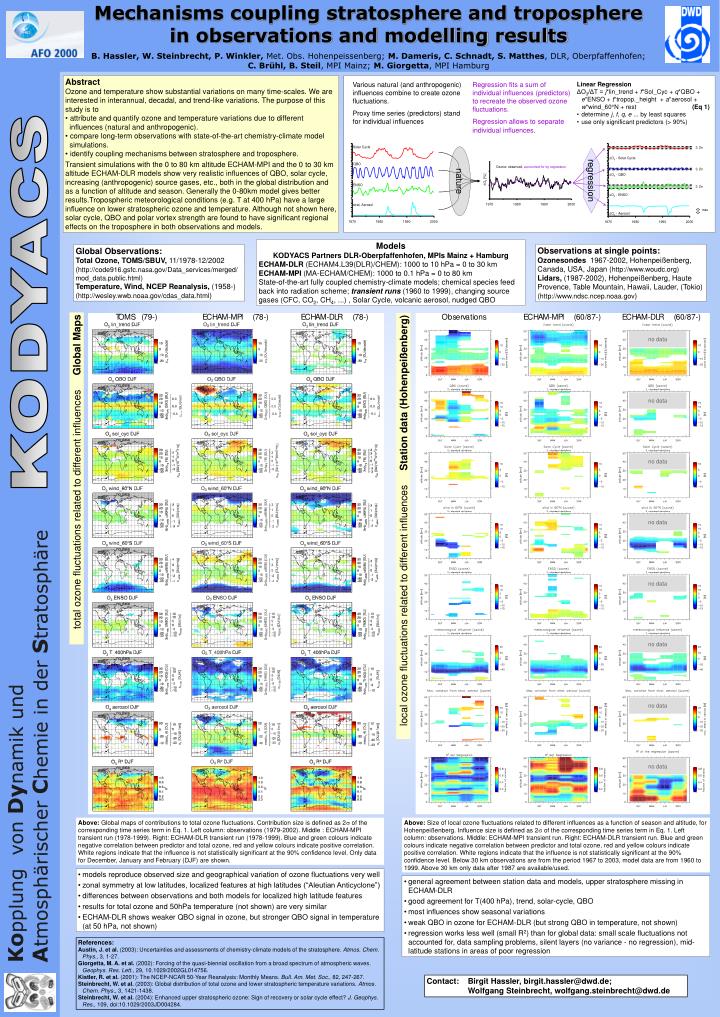
Mechanisms coupling stratosphere and troposphere in observations and modelling results B. Hassler, W. Steinbrecht, P. Winkler, Met. Obs. Hohenpeissenberg; M. Dameris, C. Schnadt, S. Matthes, DLR, Oberpfaffenhofen; C. Brühl, B. Steil, MPI Mainz; M. Giorgetta, MPI Hamburg nature Various natural (and anthropogenic) influences combine to create ozone fluctuations. Proxy time series (predictors) stand for individual influences Regression fits a sum of individual influences (predictors) to recreate the observed ozone fluctuations. Regression allows to separate individual influences. • Linear Regression • ΔO3/ΔT = j*lin_trend + f*Sol_Cyc + q*QBO + e*ENSO + t*tropop._height + a*aerosol + w*wind_60°N + rest (Eq 1) • determine j, f, q, e ... by least squares • use only significant predictors (> 90%) regression no data no data no data no data no data no data no data no data • Abstract • Ozone and temperature show substantial variations on many time-scales. We are interested in interannual, decadal, and trend-like variations. The purpose of this study is to • attribute and quantify ozone and temperature variations due to different • influences (natural and anthropogenic). • compare long-term observations with state-of-the-art chemistry-climate model • simulations. • identify coupling mechanisms between stratosphere and troposphere. • Transient simulations with the 0 to 80 km altitude ECHAM-MPI and the 0 to 30 km altitude ECHAM-DLR models show very realistic influences of QBO, solar cycle, increasing (anthropogenic) source gases, etc., both in the global distribution and as a function of altitude and season. Generally the 0-80km model gives better results.Tropospheric meteorological conditions (e.g. T at 400 hPa) have a large influence on lower stratospheric ozone and temperature. Although not shown here, solar cycle, QBO and polar vortex strength are found to have significant regional effects on the troposphere in both observations and models. Models KODYACS Partners DLR-Oberpfaffenhofen, MPIs Mainz + Hamburg ECHAM-DLR (ECHAM4.L39(DLR)/CHEM):1000 to 10 hPa = 0 to 30 km ECHAM-MPI (MA-ECHAM/CHEM): 1000 to 0.1 hPa = 0 to 80 km State-of-the-art fully coupled chemistry-climate models; chemical species feed back into radiation scheme; transient runs (1960 to 1999), changing source gases (CFC, CO2, CH4, ...) , Solar Cycle, volcanic aerosol, nudged QBO Observations at single points: Ozonesondes 1967-2002, Hohenpeißenberg, Canada, USA, Japan (http://www.woudc.org) Lidars, (1987-2002), Hohenpeißenberg, Haute Provence, Table Mountain, Hawaii, Lauder, (Tokio) (http://www.ndsc.ncep.noaa.gov) Global Observations: Total Ozone, TOMS/SBUV, 11/1978-12/2002 (http://code916.gsfc.nasa.gov/Data_services/merged/ mod_data.public.html) Temperature, Wind, NCEP Reanalysis, (1958-) (http://wesley.wwb.noaa.gov/cdas_data.html) total ozone fluctuations related to different influences Global Maps local ozone fluctuations related to different influences Station data (Hohenpeißenberg) Above: Global maps of contributions to total ozone fluctuations. Contribution size is defined as 2 of the corresponding time series term in Eq. 1. Left column: observations (1979-2002). Middle : ECHAM-MPI transient run (1978-1999). Right: ECHAM-DLR transient run (1978-1999). Blue and green colours indicate negative correlation between predictor and total ozone, red and yellow colours indicate positive correlation. White regions indicate that the influence is not statistically significant at the 90% confidence level. Only data for December, January and February (DJF) are shown. Above: Size of local ozone fluctuations related to different influences as a function of season and altitude, for Hohenpeißenberg. Influence size is defined as 2 of the corresponding time series term in Eq. 1. Left column: observations. Middle: ECHAM-MPI transient run. Right: ECHAM-DLR transient run. Blue and green colours indicate negative correlation between predictor and total ozone, red and yellow colours indicate positive correlation. White regions indicate that the influence is not statistically significant at the 90% confidence level. Below 30 km observations are from the period 1967 to 2003, model data are from 1960 to 1999. Above 30 km only data after 1987 are available/used. • models reproduce observed size and geographical variation of ozone fluctuations very well • zonal symmetry at low latitudes, localized features at high latitudes (“Aleutian Anticyclone”) • differences between observations and both models for localized high latitude features • results for total ozone and 50hPa temperature (not shown) are very similar • ECHAM-DLR shows weaker QBO signal in ozone, but stronger QBO signal in temperature (at 50 hPa, not shown) • general agreement between station data and models, upper stratosphere missing in ECHAM-DLR • good agreement for T(400 hPa), trend, solar-cycle, QBO • most influences show seasonal variations • weak QBO in ozone for ECHAM-DLR (but strong QBO in temperature, not shown) • regression works less well (small R2) than for global data: small scale fluctuations not accounted for, data sampling problems, silent layers (no variance - no regression), mid-latitude stations in areas of poor regression References: Austin, J. et al. (2003): Uncertainties and assessments of chemistry-climate models of the stratosphere. Atmos. Chem. Phys., 3, 1-27. Giorgetta, M. A. et al. (2002): Forcing of the quasi-biennial oscillation from a broad spectrum of atmospheric waves. Geophys. Res. Lett., 29, 10.1029/2002GL014756. Kistler, R. et al. (2001): The NCEP-NCAR 50-Year Reanalysis: Monthly Means. Bull. Am. Met. Soc., 82, 247-267. Steinbrecht, W. et al. (2003): Global distribution of total ozone and lower stratospheric temperature variations. Atmos. Chem. Phys., 3, 1421-1438. Steinbrecht, W. et al. (2004): Enhanced upper stratospheric ozone: Sign of recovery or solar cycle effect? J. Geophys. Res., 109, doi:10.1029/2003JD004284. Contact: Birgit Hassler, birgit.hassler@dwd.de; Wolfgang Steinbrecht, wolfgang.steinbrecht@dwd.de