NONPARAMETRIC STATISTICS

1. NONPARAMETRIC STATISTICS Vonnet Estaris, RND

2. Nonparametric Statistics • or distribution-free statistics is used when the population from which the samples are selected is not normally distributed. • This can also be used to test hypotheses that do not involve specific population parameters such as μ, σ, or ρ.

3. Advantages There are five advantages that nonparametric methods have over parametric methods: • They can be used to test population parameters when the variable is not normally distributed. • They can be used when the data is nominal or ordinal. • They can be used to test hypotheses that do not involved population parameters. • In most cases, the computations are much easier than those for the parametric counterparts. 5. They are easy to understand.

4. Disadvantages There are three disadvantages of nonparametric methods: • They are less sensitive than the parametric counterparts when the assumptions of the parametric methods are met. • They tend to use less information than the parametric tests. 3. They are less efficient than their parametric counterparts when the assumptions of the parametric methods are met.

5. Ranking • Many nonparametric tests involve the ranking of data, that is, the positioning of a data value in a data array according to some rating scale. Ranking is an ordinal variable.

6. For example, suppose a judge decides to rate five speakers on an ascending scale to 1 to 10, with 1 being the best and 10 being the worst, for categories such as voice, gestures, logical presentation and platform personality. The ratings are shown in the chart.

7. The rankings are shown next. What happens if two or more speakers receive the same number of points? Suppose the judge awards points as follows:

8. The speakers are then ranked as follows: When there is a tie for two or more places, the average of the ranks must be used. In this case, each would be ranked as: 2 + 3 5 2.5 = = 2 2

9. Sign Test • The sign test is a nonparametric test that can be used with a single group using the median rather than the mean. • For example, we can ask: Did the children in the study by Dennison and colleagues have the same median level energy intake as the 1286 kcal reported in the NHANES III study? (Because we do not know the median in the NHANES data, we assume for this illustration that the mean and median values are the same.

11. If the median of the population of 2-year-old children is 1286, the probability is 0.50 that the any observation is less than 1286. (The probability is also 0.50 that any observation is greater than 1286). We count the number of observations less than 1286 and can use binomial distribution with π = 0.50. The table contains the data on the energy level in 2-year-olds ranked from lowest to highest. Fifty-seven 2-year-olds have energy lower than 1286 and 37 have higher energy levels. The probability of observing X = 57 out of n = 94 values less than 1286 using the binomial distribution.

12. Step 1. The null alternative hypothesis are; H0 : The population median energy intake level in 2- year old children is 1286 kcal, MD = 1286. H1 : The population median energy intake level in 2- year-old children is not 1286 kcal, or MD ≠ 1286. • Step 2. Assuming energy intake is not normally distributed, • the appropriate test is the sign test; and because the • sample size is large, we can use z distribution. z = |X – nπ| - (1/2) √ nπ (1-π)

13. X = number of children with energy levels less than 1286 • n = total number of children • π = probability is 0.5, to reflect the 50% chance that the observation is less than (or greater than) the median. • Step 3. We use α = 0.05 so we can compare the results with those found in the t test. • Step 4. The critical value of the z distribution for α = 0.05 is ± 1.96. So, if there is less than –1.96 or greater than +1.96, we will reject the null hypothesis of no difference in median levels of energy intake.

14. Step 5. The calculations are z = |57 – 94(0.5)| - 0.5 √ 94(0.5) (1-0.5) = |57 – 47| - 0.5 4.85 = 9.5 4.85 = 1.96 • Step 6. The value of the sign test is 1.96 and is right on • the line with ±1.96. It is traditional that we do not reject • the null hypothesis unless the value of the test statistics • exceeds the critical value.

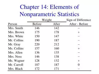
15. Wilcoxon Signed-Rank Test • When the samples are dependent, as they would be in before-and-after test using the same subjects, the Wilcoxon signed-rank test can be used in place of the t test for dependent samples.

16. Ex. In a large department store, the owner wishes to see whether the number of shoplifting incidents per day will change if the number of uniformed security officers is doubled. A sample of 7 days before security is increased and 7 days after the increase shows the number of shoplifting incidents.

17. Is there enough evidence to support the claim, at α = 0.05, that there is a difference in the number of shoplifting incidents before and after the increase in security? • Solution: Step 1. State the hypotheses and identify the claim. H0 : There is no difference in the number of shoplifting incidents before and after the increase in security. H1 : There is a difference in the number of shoplifting incidents before and after the increase in security. (claim) Step 2. The critical value of the z distribution for α = 0.05 is 2. So, if there is less than –2 or greater than +2, we will reject the null hypothesis of no difference in the number of shoplifting incidents before and after the increase in security.

18. a. Make a table as shown here. b. Find the differences (before and after), and place the values in the Difference column.

19. c. Find the absolute value of each difference, and place the results in the Absolute value column. (The absolute value of any number except 0 is the positive value of the number. Any differences of 0 should be ignored.)

20. d. Rank each absolute value from the lowest to highest, and place the rankings in the Rank column. In case of a tie, assign the values that rank plus 0.5.

21. e. Give each column plus or minus sign, according to the sign in the Difference column.

22. f. find the sum pf the positive ranks and the sum of the negative ranks separately. Positive rank sum (+3.5) + (+5) + (+6) + (3.5) + (+7) = +25 Negative rank sum (-1.5) + (-1.5) = -3 g. Select the smaller of the absolute values of the sums (|-3|), and use this absolute value as the test value ws. In this case, ws. = |-3| = 3 Step 4. Make the decision. Reject the null hypothesis if the test value is less than or equal to the critical value. In this case, 3 > 2; hence, the decision is not to reject null hypothesis. Step 5. Summarize the results. There is not enough evidence to support the claim that there is difference in the number of shoplifting incidents. Hence, the security increase probably made no difference in the number of shoplifting incidents.

23. The rationale behind the signed-rank test can be explained by a diet sample. If the diet is working, then the majority of the postweights will be smaller then the preweights. When the postweights are subtracted from the preweights, the majority of the sign will be positive, and the absolute value of the sum of the negative will be small. This sum will probably be smaller than the critical value obtained, and the null hypothesis will be rejected. On the other hand, if the diet does not work, some people will gain weight, other will lose some weight and still other people will remain about the same weight. In this case, the sum of the positive ranks and the absolute value of the negative ranks will approximately equal and will be about one-half of the sum of the absolute value of all the ranks. In this case, the smaller of the absolute values of the two sums will still be larger than the critical value obtained and the null hypothesis will not be rejected.