Download
1 / 10

E N D
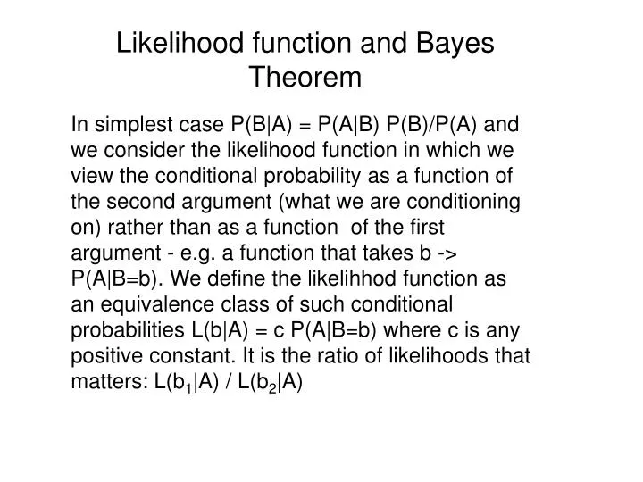
In simplest case P(B|A) = P(A|B) P(B)/P(A) and we consider the likelihood function in which we view the conditional probability as a function of the second argument (what we are conditioning on) rather than as a function of the first argument - e.g. a function that takes b -> P(A|B=b). We define the likelihhod function as an equivalence class of such conditional probabilities L(b|A) = c P(A|B=b) where c is any positive constant. It is the ratio of likelihoods that matters: L(b1|A) / L(b2|A) Likelihood function and Bayes Theorem
For the case of a probability density function with a parameter c for some observation, f(x;c), the likelihood function is L(c|x) = f(x;c) which is viewed as a function of x with c fixed as a pdf but as a function of c with x fixed as a likelihood. The likelihood is not a pdf. Example - coin toss - p=P(H) so P(HHH) = p3 and P(HHH| p = .5) = 1/8 = L(p=.5|HHH) but this does not say the probability the coin is fair, given HHH is 1/8. Can view this as having a whole collection of coins, and if you believe it is close to a “fair” collection, then P(p is “near” .5) is close to 1. This would inform the prior distribution you choose.
If we view this as likelihood of data given some hypothesis, Bayes becomes The ratio in the bottom is the odds ratio - if this is near 1 for all hypotheses then posterior s essentially same as prior - we’ve learned nothing. Best if it is near 1 for one hypothesis and small all others.
Bayesian squirrel - 2 large areas with squirrel burying all its food at location 1 w.p. p1 and all at location 2 w.p. p2 (p1 + p2 = 1) si = P(find food in location i|search location i and squirrel did bury food there) Then assume squirrel searches location with highest value of sipi . Question: If squirrel searches location 1 and doesn’t find food there, should it switch to searching location 2 the next day?
If p1’ is posterior then So use this to update the p1 and p2 each day, choose the location with highest pisi to search on the next day and repeat. The table in the book is the case for unsuccessful search - if squirrel does find food in the location a similar procedure updates the pi for the next day but in this case since the squirrel finds food there the posterior p1 = 1
The Fisher lament example is meant to show that there are cases when if we use prior knowledge, we get results that are non-intuitive if we don’t take a Bayesian view - e.g. the standard frequentist view would put all the probability mass at 0 or 1 no matter what we observe When there is a discrete number of hypotheses the two approaches are essentially the same (but often there is a continuous parameter so this doesn’t apply) but there is a problem with specifying priors if there are no observations.
Binomial Case and conjugate priors (infested tree nuts). If sample S nuts and i are infested with prob p of any nut being infested, gives a binomial form for likelihood. Then finding the posterior involves integrating this over some prior pdf for p and if we choose this prior to be a Beta Distribution (so it is over [0,1]) then he shows in the text that the posterior is also a Beta Distribution with updated parameters - this is called a conjugate prior you get the same family of distribution for posterior as the prior
Once you have a posterior, you can find the Bayesian confidence interval for a parameter in a distribution - e.g. you can get an estimate of how confident you are that the “true” parameter for a model falls in some range - just as you do with any distribution. The influence of the prior distribution can be readily overwhelmed by new data - illustrated in Fig 9.2 and the shape of the posterior may not be affected greatly by the shape of the prior - Fig 9.3. These illustrate that new data have great impact.
The generalization of Bayes for continuous densities is that we have some density f(y|) where y and are vectors of data and parameters with being sampled from a prior (|) where the are hyperparameters. If is known then Bayesian updating is If is not known then updating depends upon a distribution h()the hyperprior
The in this might specify how the parameters vary in space or time between observations which have some underlying stochasticity. One possible approach is to estimate the for example by choosing it to maximize the marginal distribution of the data as a function of by choosing it to maximize Giving an estimate and an estimated posterior This is called an empirical Bayes approach