Download
1 / 82
850 likes | 1.11k Views
Model Based Safety Analysis and Verification of Cyber-Physical Systems. PhD Dissertation Defense b y Ayan Banerjee. Advisor: Dr. Sandeep K.S. Gupta Committee Members: Dr. Radha Poovendran Dr. Georgios Fainekos Dr. Ross Maciejewski. Sponsors: . Outline. Research focus

E N D
Model Based Safety Analysis and Verification of Cyber-Physical Systems PhD Dissertation Defense by Ayan Banerjee Advisor: Dr. Sandeep K.S. Gupta Committee Members: Dr. RadhaPoovendran Dr. GeorgiosFainekos Dr. Ross Maciejewski Sponsors:
Outline • Research focus • Proving safety properties of cyber-physical interactions • Architectural modeling • Brief overview of dynamic contexts and software synthesis • Summary/Conclusions/Future research directions
Research Focus Operating Systems Software Engineering Problems Web infrastructure energy cost Cooling aware scheduling Unifying frameworks Low-cost safe medical devices Reliable and low energy communication Long-term dependable smart infrastructure Context Awareness Networking Physiological signal-based resource efficient communication Effect of contexts on safety, security, and sustainability Interactions between computing and physical domains
Common System Model Computing System Physical System Continuous physical process Computing Requirements Reliability Accuracy Throughput Latency Safety Physical Requirements Safety Energy efficiency Low carbon footprint Multi-dimensional Partial Differential Equations Actuator Discrete Control Algorithm Sensor Dynamic contexts Unintended Side Effects Random Processes Discrete Control Algorithm Cyber-Physical Interactions (CPI) Spatio-Temporal Aggregate Effects Dynamic Contexts Systems with context driven spatio-temporal, aggregate effects are cyber-physical systems (CPS) How can we assure safety under CPI?
Related Research on Safety Physical domain Computing domain Fixed operating mode Temporal/spatio-temporal dynamics Time domain discrete operation Discrete physical modeling • Control systems (temporal) • Computational fluid dynamics • Experimentation • Linear time invariant theory • Static testing • Correctness proofs • Model checking • Symbolic execution Assumptions lead to unprecedented fatalities Time domain discrete dynamics Context driven continuous spatio-temporal aggregate effects Safety of the physical environment from effects of CPI
Thesis Focus Model based safety analysis and verification under context driven spatio-temporal aggregate cyber-physical interactions Non-invasive Comprehensive Low-cost Early feedback Contribution: Hybrid models of CPI, theoretical and simulation based analysis, and automated synthesis of implementation from models Continuous dynamics Safety guarantees + Discrete domain Discrete states + State based mathematical models Continuous domain Fast simulations Dynamic contexts Synthesis of software Architectural models
Outline • Research focus • Proving safety properties of cyber-physical interactions • Architectural modeling • Brief overview of dynamic contexts and software synthesis • Summary/Conclusions/Future research directions
CPS System Model Discrete Controller Physical System Observable system properties Control algorithm configuration Control information to change physical dynamics m – modes n –system properties Variation of system properties over space and time Physical processes Spatio-Temporal Dynamics • Safety Properties • Thresholds on the system properties • Discrete state: mode of a controller (m in number) • Continuous state: a point in the Rnn-dimensional real space • Reach set: the values that system properties can assume Unsafe States v1 Reach Set Intersection indicates safety violation v2
Challenges of State Based Modeling • Hybrid nature: discrete control algorithm + continuous dynamics • Dynamics are free boundary problems [Cortazar’05] • Differential equations may not have closed form solutions • Spatio-temporal dynamics: • Multi-dimensional variation • Aggregate effects: networked operation causes aggregation of CPI • New partial differential equations • Spatial extent of aggregate effects vary over time Drug concentration for multi-channel infusion Infusion sites Y - Axis Time = 10s Time = 100s Time = 500s X - Axis
Drawbacks of Current Techniques • Reachability analysis assumes infinite precision in estimating continuous dynamics [Girard’08] • Only holds for linear time-invariant first order temporal dynamics [Girard’08] • Time bound reachability analysis • Limited to temporal dynamics [Kim’12] • Spatial networks of hybrid automata • Requires fixed spatial boundaries[Schafer’09,Bartocci’08,Ghosh’05,Yong’03] How can we capture spatio-temporal aggregate effects?
Spatio-Temporal Hybrid Automata • A hybrid automata with spatio-temporal continuous dynamics • Commonly occurring spatio-temporal continuous dynamics • Bioheat model: Penne’s bioheat equation [Pennes’48] • Infusion model: diffusion equation [Jackson’00] • Navier strokes equation is also of the same form • Heat recirculation inside a data center Linear 2nd order partial differential equation Consider Linear 1-D space STHA (L1STHA)
L1STHA Definition System Model Control information reset functions Discrete Controller Physical System Control algorithm configuration System properties vary in continuous state space 2 –system properties 2 – modes Mode change governed by invariants Physical processes Spatio-Temporal Dynamics Continuous State Space Mode Mode Inv2 v1 Inv1 v2 Continuous Variables = v1 , v2
L1STHA Execution Model 200 180 160 140 120 100 80 60 40 20 0 0 5 10 15 20 25 30 35 40 45 50 0 5 10 15 20 25 30 35 40 45 50 • Trajectory: solution of PDE of a mode li • Execution: concatenation of trajectories – spatial or temporal • Modetransition: when trajectory crosses invariant sets – spatial or temporal • Deterministic and transversal – no zeno behavior (DTL1STHA) [Lamperski’08] • Initial state, v0 , at a given space point at t = 0s • Initial configuration, V0 , space map at t = 0s • Reach set:set ofvalues for continuous variables for any execution Correction bolus mode Insulin infusion pump Spatial execution Basal mode Temporal discrete transition Spatial discrete transitions Temporal execution Glucose Concentration mg/dl Braking mode X-axis Coordinate
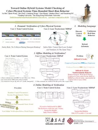
Reachability Analysis Find the continuous states reached by the DTL1STHA for any time and space The problem is undecidable ε approximation of reach set using exact solutions in a continuous time domain Set of initial states Traditional temporal approach Execution Only feasible if spatio-temporal dynamics can be solved with infinite precision Free boundary problems - may not have closed form solution Sampled time and space bounded approximation analysis
Approximation Methodology Hausdorff Distance Find the shortest distance of a point from P to Q Find the maximum among them P Q Q3= (δ,δ) Q4= (- δ,δ) dH (S,Q6) = max(δ-0,gδ-0) = δ S Q5= (fδ,gδ) Q6= -δ,-gδ dH (S,Q5) = max(fδ-0,gδ-0) < δ dH is the Hausdorff distance δ neighborhood 0,0 Q2= (δ,-δ) Q1 = (-δ,-δ) neighborhood approximation Convex hull
Time and Space Bound Reachability Sample time hx and space ht Start with a δ neighborhood of the initial configuration Approximate the reach set at each discrete step by Determine δ and such that the overall error in reach set estimation is less than ε neighborhood Reach set Inv1 ε reach set Convex Hull Inv0 vert3 vert2 v0 vert4 vert1 Approximate trajectory Image of the vertex Transition δ neighborhood What makes this possible?
Lemmas, Theorems, and Proofs Lemma 1: Finding sampling of time hx and space ht such that the trajectory is within ε boundary of the sampled states in each interval Proof: Requires solution of the PDE with a finite error margin Lemma 2: If we consider a single mode DTL1STHA, then there exists a and such that the reach set computed by the convex hull method is an ε reach set Proof: This ignores transitions between modes and the change in dynamics due to mode change Transitions can be ignored: if back and forth transition occurs within an interval Infeasible transitions can occur: ε reach set may intersect multiple modes leading to non-determinism even for a one mode case
Tackling Transitions Lemma 3: If the trajectory of a DTL1STHA satisfies deterministic and transversal transition conditions, then there exists and less than the values given in Lemma 2, such that the transition will not be ignored or no infeasible transition can occur Proof: Requires formally defining deterministic and transversal transitions and over- approximating the rate of variation of the continuous states The reachability analysis can start with and suggested in Lemma 2 Iterative transition tracking: on an infeasible transition, reduce the values by a fraction α and restart Theorem 1: The convex hull method of image computation combined with the iterative transition tackling method finishes in finite time and outputs the ε reach set. Proof: Lemma 2 states that the convex hull computation method outputs the reach set. Lemma 3 states that for each transition, there exist finite and which the transition tackling method captures.
Reachability Analysis of Infusion Pumps • Analysis performed for five control parameters: • a) infusion increment rate, b) control input delay, c) drug concentration set point, d) sample interval, e) bolus value • For each configuration, reachability analysis is performed • 2D projections of a 5D graph • Islands indicate safe optimal configurations Publications: ICCPS’13 (under review), Isabel’11, AAMI Horizons’13 (under review)
Outline • Research focus • Proving safety properties of cyber-physical interactions • Architectural modeling • Brief overview of dynamic contexts and software synthesis • Summary/Conclusions/Future research directions
Related Research Efforts CPS Modeling Requirements Existing Modeling Approaches Modeling Cyber Entities Cyber Entities Software design tools (e.g. UML, PetriNets, AADL) Application Software can address software and operational safety Embedded system design tools (e.g. AADL, Pspice) Network of Computing Units Modeling Cyber-Physical Interactions Actuators Intended Interaction (Karsai’08) Sensors can address interaction and operational safety Unintended Interactions Physical Behavior Physical Processes can address mechanical safety and biocompatibility Physical process modeling tools (e.g. SysML, Simulink, Flovent) Physical Environment
Architectural Model of CPS Computing Operations Physical Operations Spatio-temporal CPI Aggregate Effects
Example: Body Sensor Networks 312.5 312 311.5 311 310.5 0.04 0.03 0.04 0.03 0.02 0.02 0.01 0.01 0 0 EEG EKG BP SpO2 Base Station Unintended interactions (heating effects) Wearable Sensor Nodes Aggregate Effects Base Station Thermal Map of Human Body Communication Range Motion Sensor Intended Interactions(communication range) Penne’s Bioheat Equation Temperature K Power circuitry Heat Accumulated Heat transfer by convection Metabolism Heat transfer by conduction Heat transfer by radiation X coordinate Y coordinate
BSN Modeling with GCPS 0 0 0.005 0.005 0.01 0.01 0.015 0.015 0.02 0.02 0.025 0.025 0.03 0.03 0.035 0.035 0.04 0 0.005 0.01 0.015 0.02 0.025 0.03 0.035 0.04 0.04 0 0.005 0.01 0.015 0.02 0.025 0.03 0.035 0.04 Computing Properties: sampling frequency Physical Monitored Parameter: temperature Physical Properties: heat dissipation Region of Impact: spatial region affected by heat ROIm Physical Dynamics: Penne’s bioheat equation Region of Interest: communication range Computing Monitored Parameter: packet delivery ratio ROIm Region Boundary: constraints on PDE Change in Region of Impact Region Boundary Computing Unit Change in Region Boundary Region of Impact Region Boundary Region of Interest LCPS at time = 1100s LCPS at time = 24hrs Projection of the thermal distribution on the Y axis where the temperature is maximum 312.5 312.5 312.5 Tsafe 312 312 312 Tth Tth Temperature in K 311.5 311.5 311.5 311 311 311 N1 N1 N1 I1 310.5 310.5 310.5 I1 Unsafe I1 N1 N1 310 310 310 0.04 0 0.01 0.02 0.03 0 0.01 0.02 0.03 0.04 0 0.01 0.02 0.03 0.04 (b) X spatial dimension after 1100 s (c) X spatial dimension after 24 hrs (a) X spatial dimension after 40 s Thermal map evolution over time for a single sensor
Aggregate Effects 1 18 16 14 12 10 8 6 4 2 0 2 3 4 5 6 7 8 9 Aggregate Effects: occurs when the ROIm of two sensors overlap 1 18 16 14 12 10 8 6 4 2 0 Dynamics for aggregate effects may have different forms than the individual ones 2 3 Aggregate Penne’s Bioheat Equation: summation of power and SAR values 4 5 6 7 8 Unsafe temperature zones 9 Dynamics for aggregate effects can have complex forms such as simultaneous solutions of non-linear PDEs, as in the case of infusion pumps ROIm 1 ROIm 2 How can we analyze a CPS for such complex aggregate effects? ROIm 1 Overlap ROIm 2
Analysis Challenges • The physical processes are free boundary problems • There is no fixed spatial boundary • Spatial discretization techniques are not intuitively applicable • At each LCPS, we need to determine the spatial region for each time instant, where effects of CPI are observed • Computation of aggregate effects becomes complex • For each pair of LCPS, we need to compute the intersection of ROIm • We then need to solve new PDEs in the intersecting regions • PDEs for aggregate effects have to be specified in the GCPS model
GCPS Implementation - CPSDAS • CPS-DAS input: • It consists of a) requirements model, b) GCPS model, and c) analysis parameters • Implemented in Architectural Analysis and Design Language (AADL) • Analyzer implemented in OSATE as an Eclipse plug-in Publications: ACM TECS’12
Outline • Research focus • Proving safety properties of cyber-physical interactions • Architectural modeling • Brief overview of dynamic contexts and software synthesis • Summary/Conclusions/Future research directions
Effect of Using Different Mobility Models on Safety Conclusions • Indoor PDR is greater than the outdoor PDR [Natarajan’09] • Outdoor excursions increase the chance of packet drop • Upon loss of control information, the pump retains previous infusion rate Indoor PDR = 0.8 1500 Levy Walk 1 Levy Walk 2 Outdoor PDR = 0.4 Random Way Point Probability of outdoor excursions = 0.7 1000 Drug concentration in ug/l 500 Conclusions on safety depend on models of mobility 0 0 1 2 3 4 5 Time in minutes How can we analyze safety under dynamic contexts? Publications: Percom’12, TMC (under preperation)
Health-Dev: Medical CPS Synthesis Wireless Health System Design Tool Design Steps Specification of WHS using UI Model Generate Code Code Download the code Publications: BSN’12, WHS’12
Outline • Research focus • Proving safety properties of cyber-physical interactions • Architectural modeling • Brief overview of dynamic contexts and software synthesis • Summary/Conclusions/Future research directions
Summary of Contributions Models, Analysis, and Synthesis CPS System Thermal Effects Power Requirements Analysis 17 collaborative publications, 2 first author Profiling Drug Effects Safety Requirements STHA Model Model Development Architectural Models 2 conferences, 3 journals, all first author, 2 under review Model Analysis Reachability Analysis Simulation Analysis Verifier Model Synthesis 2 conference, first author Software Synthesis Experimentation
Conclusions • Multi-dimensional spatio-temporal aggregation impose hard challenges in model based safety verification of CPS. • This thesis proposes methodologies to handle aggregate CPI under dynamic contexts and prove theoretical properties. • Validation of the techniques are performed on empirical data obtained from experiments reported in publications. • A major focus in the next few years will be to perform clinical studies to validate the approaches.
Future Works • Hierarchical models • To capture random events in a hybrid system • Multi-dimensional space reachability analysis • CPSes with active physical systems • Interplay of human and robot • Physical environment is no more a passive entity
References • [Cortazar05] C. Cortazar, M. Elgueta, and J. D. Rossi, “A nonlocal diusion equation whose solutions develop a free boundary,” Annales Henri Poincare, vol. 6, pp. 269–281, 2005, 10.1007/s00023-005-0206-z. [Online]. Available: http://dx.doi.org/10.1007/s00023-005-0206-z • [Girard08] A. Girard and C. Guernic, “Zonotope/hyperplane intersection for hybrid systems reachability analysis,” in Proceedings of the 11th international workshop on Hybrid Systems: Computation and Control, ser. HSCC ’08. Berlin, Heidelberg: Springer-Verlag, 2008, pp. 215–228. [Online]. Available: http://dx.doi.org/10.1007/978-3-540-78929-1 16 • [Kim12] K.-D. Kim, S. Mitra, and P. R. Kumar, “Bounded epsilon-reach set computation of a class of deterministic and transversal linear hybrid automata,” CoRR, vol. abs/1205.3426, 2012 • [Schafer09] A. Schafer and M. John, “Conceptional Modeling and Analysis of Spatio-Temporal Processes in Biomolecular Systems,” in Sixth Asia-Pacific Conference on Conceptual Modelling (APCCM 2009), ser. CRPIT, S. Link and M. Kirchberg, Eds., vol. 96. Wellington, New Zealand: ACS, 2009, pp. 39–48. • [Bartocci08] E. Bartocci et al, “Spatial Networks of Hybrid I/O Automata for Modeling Excitable Tissue,” Electronic Notes in Theoretical Computer Science (ENTCS), vol. 194, no. 3, pp. 51–67, 2008. • [Ghosh05] R. Ghosh and C. Tomlin, “A query-based technique for interpreting reachable sets for hybrid automaton models of protein feedback signaling,” in Proceedings of the American Control Conference, June 2005, pp. 4417–4422. • [Yong03] Q. Yong, W. Ying-Jie, and J. Li-Min, “Hybrid cellular automata model for railway transportation system and its implementation on GIS,” in Intelligent Vehicles Symposium, June 2003, pp. 543 – 546. • [Pennes48] H. H. Pennes, “Analysis of tissue and arterial blood temperature in the resting human forearm,” in Journal of Applied Physiology, vol.1.1, 1948, pp. 93–122. • [Jackson00]T. L. Jackson and H. M. Byrne, “A mathematical model to study the eects of drug resistance and vasculature on the response of solid tumors to chemotherapy,” Mathematical Biosciences, vol. 164, no. 1, pp. 17 – 38, 2000. • [Grgoire98]N. Grgoire and M. Bouillot, “Hausdor distance between convex polygons.” [Online]. Available: http://cgm.cs.mcgill.ca/godfried/teaching/cg-projects/98/normand/main.html • [Alt90] H. Alt, J. Blmer, and H. Wagener, “Approximation of convex polygons,” in Automata, Languages and Programming, ser. Lecture Notes in Computer Science, M. Paterson, Ed. Springer Berlin / Heidelberg, 1990, vol. 443, pp. 703–716, .[Online]. Available: http://dx.doi.org/10.1007/BFb0032068
References • [Lamperski08] A. Lamperski and A. Ames, “On the existence of zeno behavior in hybrid systems with non-isolated zenoequilibria,” in Decision and Control, 2008. CDC 2008. 47th IEEE Conference on, dec. 2008, pp. 2776 –2781. • [Karsai08] Karsai et al, “Model-integrated development of cyber-physical systems,” in SEUS’08: Proceedings of the 6th IFIP WG 10.2 international workshop on Software Technologies for Embedded and Ubiquitous Systems. Berlin, Heidelberg: Springer- Verlag, 2008, pp. 46–54. • [Rhee08]I. Rhee, M. Shin, S. Hong, K. Lee, and S. Chong, “On the levy-walk nature of human mobility,” in INFOCOM 2008. The 27th Conference on Computer Communications. IEEE, april 2008, pp. 924 –932. • [Natarajan09] A. Natarajan, B. de Silva, K.-K. Yap, and M. Motani, “To hop or not to hop: Network architecture for body sensor networks,” in Sensor, Mesh and Ad Hoc Communications and Networks, SECON ’09. 6th Annual IEEE Communications Society Conference on, june, pp. 1 –9. • [Banerjee11] S. Nabar, A. Banerjee, S.K.S. Gupta, and R. Poovendran,GeM-REM: Generative Model-driven Resource-efficient ECG Monitoring in Body Sensor Networks , Body Sensor Networks 2011, Dallas, Texas • [BK12] B. K. et al, “Control to range for diabetes: Functionality and modular architecture,” Journal of diabetes Science and Technology, 2012 • [Graseby] S. Medical, “Graseby 3300 technical manual,” http://www.frankshospitalworkshop. com/equipment/documents/infusion_pumps/service_manuals/Graseby_3300_Syringe_Pump_-_Service_manual.pdf. • [Airbus] http://catless.ncl.ac.uk/Risks/8.77.html#subj6 • [Jetley06]R. Jetley, S. P. Iyer, and P. L. Jones, “A formal methods approach to medical device review,” Computer, vol. 39, no. 4, pp. 61–67, 2006. • [Arney09] D. E. Arney, R. Jetley, P. Jones, I. Lee, A. Ray, O. Sokolsky, and Y. Zhang, “Generic infusion pump hazard analysis and safety requirements version 1.0,” 2009. [Online]. Available: http://repository.upenn.edu/cis_reports/893
Example – Infusion Pump • Three modes – Braking, Basal, and Correction Bolus [BK12] • Braking mode when glucose concentration is less than 20 mg/dl, initial conc = I01 /f • Basal mode when glucose concentration > 20 mg/dl and < 120 mg/dl, initial conc I01 • Correction bolus mode when glucose concentration > 120 mg/dl, increase conc by Ib1 Diffusion Equation Braking Basal Correction Bolus
Aggregate effects – Multi-Channel • Multi-channel infusion with two drugs – occurs when both drug concetrations are above low threshold. • Mode set is Cartesian product • Aggregate effect d3 specified to the L1STHA as a separate PDE. • L1STHA finds out where, when and how much aggregate effect Correction Bolus 1 + Braking 2 Aggregate Correction Bolus 1 + Correction Bolus 2
Model Based Engineering • Models – Simplifying abstractions of real systems • Models aide in: • Development of entire system: Model Based System Engineering • Management of processes in the system – Model Based Process Engineering • Development of the software of the system – Model Based Software Engineering Early feedback aide in removing unfavorable designs hence reduce time and effort Model Based Software Engineering Requirements Analysis Development Validation Analysis & Verification Deployment Maintenance 30% 30% 30% 100% 15% 10% Thesis focus
Model based software analysis verification Formal Models: State machine CPS System Always safe for any initial configuration Thermal Effects Power Requirements Analysis Profiling Drug effects SLOW Guaranteed Safe Speed Safety Requirements Architectural Models: Represented as a collection of components Model Development Formal Models Architectural Models Safe for a given configuration for a given time Model Analysis Reachability Analysis Simulation Analysis Verifier FAST Safe under assumptions Model Synthesis Software Synthesis Hardware Synthesis Experimentation
Related Research Models of CPSes Use of existing models Extension of existing models New models 1. Spatial Networks of hybrid automata 9,10,11 2. Hierarchical models12 3. Cellular hybrid automata13 1. Spatio-temporal event models14,15 2. Spatio-temporal mobility models16 3. Spatio-temporal databases17,18 4. Hilbertean transforms19 1. Finite State Automata1,2,3 2. Timed Automata4,5 3. Hybrid Automata6,7,8 Ignores spatio-temporal Interactions Has static assumptions on physical systems Considers fixed spatial boundaries of interactions Has no theoretical guarantees
Validation of generated code Health-Dev Maintainer BSN Developer Tools Features Time Savings: BSN with ECG and accelerometer sensors and smart phone display Health-Dev: 346 LOC/ 1895 LOC (Lines Of Code) Code Modification Time Changing sensor type in the same hardware: 1LOC/3LOC Adding a sensor: 1 AADL subcomponent typically 22 LOC / 75 LOC Adding a graphing variable in smart phone:8LOC/153LOC Adding algorithms to database: Needs to write the algorithm in the chosen programming language Code Size and RAM Consumption Programming Limitations Reduction in RAM size – Modular Code, RAM utilization is reduced Algorithm not in database cannot be specified No over-the-air reprogramming support Integer point programming, no floating point support Limited support for atomic operations Dynamic thresholding of signals not supported Increase in code size – use of pre processing directives Support for New Hardware 1. AADL property sets 2. Parser modifications 3. Link the parsed AADL properties to appropriate OS abstractions
Example: Continuous Monitoring system Sensor features InputData: indataport; OutputData: inoutdataport; end Sensor; ECG Communication via Bluetooth • Sensor components: • sensor properties, • communication handler, and • processing algorithms • BSNBench [WH’ 09] – a BSN specific benchmark suite, • Physiological signal processing algorithm, • Statistical manipulations, • Energy management algorithms systemimplementation Sensor.node1 subcomponents NodeId: data node_ids.node1; Comm: system Communication.ID0; Alg_FFT256: process Algorithm.FFT_1; Alg_PeakDetect: process Algorithm.PeakDetect_1; properties SensorParameter::SamplingFreq => 125 Hz; SensorParameter::Platform => shimmer; SensorParameter::SensorType => "ECG"; NetworkParameters::Radio => "DynamicDutyCycle"; connections AlgInput: dataportInputData -> Alg_FFT256.Input; AlgOutput: dataportAlg_FFT256.Output -> Alg_PeakDetection.Input; AlgOutput2: dataportAlg_PeakDetect.Output -> OutputData; SendData: dataport OutputData -> Comm.Send_Data; endSensor.node1; Accelerometers Mobile phone
GCPS Analysis Algorithm Input: GCPS Object, Functions to evaluate physical dynamics, Parameters of the simulation, dynamics for aggregate effects • Interactions between computing unit and physical system • for each i from 1 … n • GCPS.LCPS(i).ROIm.Physical Property = EvaluatePhysicalProperty(GCPS.LCPS(i).ROIm, AnalysisParameters) • for each i from 1 … n • GCPS.LCPS(i).ROIn.Monitored Parameter = EvaluateMonitoredParameter(GCPS.LCPS(i).ROIn, AnalysisParameters) • Interaction between different computing units • for each i from 1 … n • for each j from 1 … n • if GCPS.LCPS(i).ROIm.RB overlap with GCPS.LCPS(j).ROIm.RB then IntFm(i,j) = 1; • Else IntFm(i,j) = 0; • for each IntFm(i,j) == 1 • GCPS.LCPS(i).ROIm.Physical Property = Compute the aggregate effect in the intersecting region; • GCPS.LCPS(j).ROIm.Physical Property = Compute the aggregate effect in the intersecting region; Output: Conformity to safety requirements
Case Study I: Thermal Safety of Pulse-Oximeter • Fingertip Pulse-oximeter (from Smithsoem) deployed on index finger • Eight hours continuous operation • Sampling rate = 60 samples/sec • The control area of the fingertip skin was divided into square grids and the thermal map was calculated as shown in the Fig 3. • Results • fingertip skin did not exceed safe limits for pulse oximeter’s operating temperatures of 43.5o C. • tissue thermal damage was observed for higher operating temperatures.
Case Study 2: Medical Device Control Operation Control Inputs Bolus Request Perturbation Control Algorithms Reference drug concentration level Infusion Rate Control Error Programmed Infusion Rate Infusion Pump + - Control Actions Target Open Loop System Pharmacokinetic Model Predicted drug concentration level Feedback from human body model
Pharmacokinetic Model • A state space model is provided • The drug diffusion process using the three compartment model • Time variant dynamics • Cardio-pulmonary transport delays • Arterial blood transport delay • Input Delay 2. The hybrid model: A new pharmacokinetic model for computer controlled infusion pumps, Russel Wada et. al.
Pump Stability Stability Accuracy Short Settling Small Overshoot