Download
1 / 14
140 likes | 253 Views
Constraints on primordial non-Gaussianity using Planck simulated data. Marcos López-Caniego Andrés Curto Enrique Martínez-González Instituto de Física de Cantabria (CSIC-UC). Introduction

E N D
Constraints on primordial non-Gaussianity using Planck simulated data Marcos López-Caniego Andrés Curto Enrique Martínez-González Instituto de Física de Cantabria (CSIC-UC)
Introduction After the successful porting of the point source detection code and the SZ clusters detection code to the EGEE GRID, we are in the process of porting and testing a new application. This application is composed of two codes, one to produce Gaussian simulations of Planck and another to look for non-Gaussianity signatures in these maps using spherical wavelets. These applications are part of an ongoing project being carried out by the Observational Cosmology and Instrumentation Group at the Instituto de Física de Cantabria (CSIC-UC) on different analyses of the Cosmic Microwave Background (CMB). EGEE09, Barcelona, Spain, 24 September 2009
Motivations The Planck mission will provide CMB maps with unprecedented resolution and quality at several frequencies. Therefore, we expect to obtain the very competitive constraints on the primordial non-Gaussianity with this experiment. The study of this kind of non-Gaussianity through the study of the non-linear coupling parameter fnl has become a question of considerable interest as it can be used to discriminate different possible scenarios of the early Universe and also to study other sources of non-Gaussianity non-intrinsic to the CMB. The uncertainties on the fnl, s(fnl), depend on the cosmological model, the instrumental properties and the available fraction of the sky to be analyzed, e.g., a better estimation on fnlcan be achieved with a low instrumental noise and a high sky coverage. The constraints on fnl can be obtained using two methods: • simulations • analytical equations. EGEE09, Barcelona, Spain, 24 September 2009
The Analysis with Simulations First, 10,000 of Gaussian CMB maps are simulated and processed through the Planck instrument simulation pipeline for three frequency bands, 100, 143 and 217GHz, producing three maps per simulation. Then, these maps are combined into a single map. EGEE09, Barcelona, Spain, 24 September 2009
The Analysis with Simulations First, 10,000 of Gaussian CMB maps are simulated and processed through the Planck instrument simulation pipeline for three frequency bands, 100, 143 and 217GHz, producing three maps per simulation. Then, these maps are combined into a single map. Second, for each simulation, the combined map is convolved in harmonic space with a spherical wavelet, in this case the spherical Mexican hat wavelet (SMHW) will be used. EGEE09, Barcelona, Spain, 24 September 2009
position scale traslation • The spherical Mexican hat wavelet (SMHW) • Continuous wavelet transform EGEE09, Barcelona, Spain, 24 September 2009
The wavelet is a filter EGEE09, Barcelona, Spain, 24 September 2009
The Simulations First, 10,000 of Gaussian CMB maps are simulated and processed through the Planck instrument simulation pipeline for three frequency bands, 100, 143 and 217GHz, producing three maps per simulation. Then, these maps are combined into a single map. Second, for each simulation, the combined map is convolved in harmonic space with a spherical wavelet, in this case the spherical Mexican hat wavelet (SMHW) will be used. The convolved map, the wavelet coefficients map, will contain information about those structures of the initial map with a characteristic size R. EGEE09, Barcelona, Spain, 24 September 2009
We will repeat this process for several angular scales R between 2.9 arc minutes and about 170 degrees. Finally we use third order statistics (in a similar way as the bispectrum) to constrain the levels of non-Gaussianity of the local type which are expected to be present in Planck data. EGEE09, Barcelona, Spain, 24 September 2009
Simulation of 10.000 Gaussian maps per frequency • Input • Power spectrum of the cosmological model (~1 KB) • Instrumental beams (~1 KB) • Instrumental variance for each pixel (total ~15 MB) • Algorithm • Generate Gaussian coefficients in the sphere alm • Transform the alm to DT/T maps and add instrumental beam • Add Gaussian noise for each bolometer • Total time and memory per simulation: 5 min, 1GB of RAM • Output • 10.000 maps/frequency and 10.000 combined maps=40.000 maps • 15 MB per map => 0.6 TB • Aprox. 1000 CPU hours per scale => 30.000 CPU hours total EGEE09, Barcelona, Spain, 24 September 2009
Analysis of the 10.000 simulations • Input • Planck Gaussian simulations (15 MB each) • Algorithm • Select a set of n angular scales {Ri} • Compute the wavelet transform (5 min and 1 GB RAM each scale) • Evaluate the cubic statistics • Output • Cubic statistics: for n scales, (n+2)!/[(n-1)!3!] files (several KB per map) • Aprox. 5000 CPU hours to do the analysis of the 10.000 simulations EGEE09, Barcelona, Spain, 24 September 2009
Analytic estimation of C and a • Input • Cosmological parameters and power spectrum (several KB) • Transfer function generated by gTfast (available on-line by E. Komatsu) ~50 GB • Algorithm • Parallelize the estimation of C and a using three indices: l1, l2, l3from 0 to 3096 each • Number of CPUS: 100-200 • Total time: about 50.000 hours • Total RAM per CPU: 1 GB • Output • Each job produces a pair of a(i) and C(i) • Final a and C parameters are the sum EGEE09, Barcelona, Spain, 24 September 2009
First check: Estimate Covariance matrix in 1 scale • Evaluate the covariance with 1000 Gaussian simulations C(sims) • Evaluate the covariance matrix with the analytical expression C(theo) • Check that the analytical value for the covariance agrees with its estimator with 1000 Gaussian simulations and 1 scale • The differences are < 6% DONE Future Work: continue with the analysis of the remaining 20 scales • Estimate the covariance matrix using 21 scales with sims (~40.000 CPU hours) • Estimate the a coefficients using 21 scales analytically (~50.000 CPU hours) • Constraint fnl and compare with the bispectrum EGEE09, Barcelona, Spain, 24 September 2009