Introduction

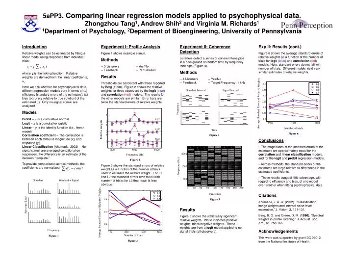
1. 5aPP3. Comparing linear regression models applied to psychophysical data. Zhongzhou Tang1, Andrew Shih2 and Virginia M. Richards1 1Department of Psychology, 2Deparment of Bioengineering, University of Pennsylvania Experiment II: Coherence Detection Listeners detect a series of coherent tone pips in a background of random time-by-frequency tone pips (Figure 4). Methods -- 4 Listeners -- Yes/No -- Feedback -- Target Frequency: 1 kHz Exp II: Results (cont.) Figure 6 shows the average standard errors of relative weights as a function of the number of trials for logit (blue) and correlation (red) models. Note: standard errors do not fall with number of trials. Different models yield very similar estimates of relative weights. Introduction Relative weights can be estimated by fitting a linear model using responses from individual trials: where g is the linking function. Relative weights are derived from the linear coefficients, j. Here we ask whether, for psychophysical data, different regression models vary in terms of (a) efficiency [standard errors of the estimates], (b) bias [accuracy relative to true solution] of the estimated s. Only no-signal stimuli are analyzed. Models Probit – g is a cumulative normal Logit – g is a cumulative logistic Linear – g is the identity function (i.e., linear model) Correlation coefficient – The correlation is between each stimulus magnitude (xij) and response (yi). Linear Classification (Ahumada, 2002) – No-signal stimuli are averaged conditional on responses, the difference is an estimate of the decision “template.” To provide comparisons across methods, the coefficients are normalized: Experiment I: Profile Analysis Figure 1 shows example stimuli. Methods -- 3 Listeners -- Yes/No -- Feedback -- Perturbation Results Thresholds are consistent with those reported by Berg (1990). Figure 2 shows the relative weights for three observers by the logit (blue) and correlation (red) models. The results for the other models are similar. Error bars are twice the standard errors of relative weights. 0.4 L4 L5 Standard Interval Signal Interval 0.35 L6 L7 0.3 Average Standard Errors of Relative Weights 0.25 0.2 Frequency 0.15 0.1 1150 1626 2300 Number of trials Relative Weights Time Figure 6. Figure 4 Conclusions – The magnitudes of the standard errors of the estimates are approximately equal for the correlation and linear classification models, and for the logit and probit regression models. – Across methods, the standard errors of the estimates are large relative to differences in the estimated coefficients. – These results suggest little advantage, with regard to efficiency and bias, of one model over another when fitting psychophysical data. Citations Ahumada, J. A. Jr. (2002). “Classification image weights and internal noise level estimation,” J. Vision, 2, 121-131. Berg, B. G. and Green, D. M. (1990). “Spectral weights in profile listening,” J. Acoust. Soc. Am., 88, 758-766. Acknowledgements This work was supported by grant DC 02012 from the National Institutes of Health. Frequency (Hz) Figure 2 Figure 3 shows the standard errors of relative weight as a function of the number of trials used to estimate the relative weight. For L1 and L2 the standard errors tend to fall with number of trials; for L3 that result is less obvious. Frequency (Hz) Standard Standard + Signal Time (ms) Figure 5 Spectrum Level Results Figure 5 shows the statistically significant relative weights. White indicates positive weights, black negative weights. These weights are from a logit model applied to no-signal trials (all observers). Average Standard Errors of Relative Weights Frequency Number of trials Figure 1 Figure 3