Download

1 / 13
140 likes | 233 Views
Small Forwarding Tables for Fast Routing Lookup. Data : 2014.04.13. Design goals and parameters. The Small Forwarding Table(SFT), In general, The small forwarding table is the compressed version of a 16-8-8 trie . Since

E N D
Small Forwarding Tables for Fast Routing Lookup Data : 2014.04.13
Design goals and parameters The Small Forwarding Table(SFT), In general, The small forwarding table is the compressed version of a 16-8-8 trie. Since SFT organizes the first 16 levels of trie in a 12-4 hierarchical Fashion, it can be also classified as a 12-4-8-8 trie. When designing the data structure used in the forwarding table, The primary goal was to minimize lookup time. To reach that goal, we simultaneously minimize two parameters. • The number of memory accesses required during lookup. • The size of the data structure.
The data structure for level 1 (1/8) The forwarding table is a representation of the binary tree spanned by all routing entries. This is called the prefix tree. it’s require that the prefix tree is complete. The forwarding table is essentially tree with three levels.
The data structure for level 1 (2/8) Nodes with a single child must be expanded to have two Children, the children added in this way are always leaves, and Their next-hop is the same as the next-hop of the closest ancestor With next hop information, or the “undefined” next-hop if no such ancestor exists.
The data structure for level 1 (3/8) • Level 1 of the data structure Image a cut through the prefix tree down to depth 16, the Cut is represented by bit-vector, with one bit per possible node at depth 16, are required fort this. When there is node in the prefix tree at depth 16, the corresponding bit in the vector is set. • Bit is set: prefix continues below the cut, called a root head. • Bit is set: a leaf at depth 16 or less, a genuine head. • Bit is unset.
The data structure for level 1 (4/8) Leaf push
The data structure for level 1 (4/8) Genuine head: bits 0, 4, 7, 8, 14, 15 root head: bits 6, 12, 13 The bit-vector is divided into bit-mask of length 16. There are
The data structure for level 1 (5/8) The head information is encoded in 16-bit pointers stored consecutively in an array (pointer group). Two bits of each pointer encode what kind of pointer it is, and 14 remaining bits either form an index into the next-hop table or an index into an array containing level two chunks
The data structure for level 1 (6/8) The code words consists of a 10bit value(r1, r2,…) and a 6bit offset (0, 3, 10, …). After four code words, the offset value might be too large to represent with 6 bits, therefore, a base index is used together with the offset to find a group of pointers. ( length of base index array element is 16bits. ) Code word array and Base index array
The data structure for level 1 (7/8) Pointer group 0 1 2 3 4 ……. Maptable
The data structure for level 1 (8/8) Searching: search the first level of the data structure.
The data structure for level 2、3 (1/2) Levels two and three of the data structure consist if chunks. A chunks covers a subtree of height 8 and can contain at most heads. A root head in level n-1 points to a chunk in level n. There are three varieties of chunks depending on how many heads the imaginary bit vector contains. When there are • 1-8 heads, the chunk is sparse and is represented by an array of the 8bits indices of the head plus eight 16-bit pointers.
The data structure for level 2、3 (2/2) • 9-64 heads, the chunk is dense. It’s represented analogously with level 1, except for the number of base indices. The difference is that only one base index is needed for all 16 code words, because 6-bits offsets can cover all 64 pointer. A total of 34bytes are needed. • 65-256 heads, the chunk is very dense. It’s represented analogously with level 1, 16 code words and 4 base indices give a total of 40bytes.