Download

1 / 20
200 likes | 418 Views
DIGITAL SPREAD SPECTRUM SYSTEMS. ENG-737. Wright State University James P. Stephens. INTERCEPT CONSIDERATIONS. Anti-Intercept (AI) Low Probability of Intercept (LPI) Low Probability of Detection (LPD) Low Probability of Exploitation (LPE) Covert Communications.

E N D
DIGITAL SPREAD SPECTRUM SYSTEMS ENG-737 Wright State University James P. Stephens
INTERCEPT CONSIDERATIONS • Anti-Intercept (AI) • Low Probability of Intercept (LPI) • Low Probability of Detection (LPD) • Low Probability of Exploitation (LPE) • Covert Communications • All refer to minimizing an interceptor’s ability to: • Detect the presence of the signal in the midst of natural noise and RFI • Locate the position of the transmitter
INTERCEPT CONSIDERATIONS • Detection relates to knowing that a signal is present • Intercept relates to having detected a signal, can you identify anything about it • Exploitation relates to being able to copy the signal well enough to intercept the message content • Interceptor’s ability to identify and exploit a signal is somewhat dependent upon: • The frequency range • Channel geometry (line-of-sight) • But mostly dependent upon SNR at the detector • LPI Radar Contrasted • Radar signal requires return path (R-4) • Typically omni-directional • Typically directed toward power reduction or limiting the response time of the RWR • LPI to a communicator is not being detected at all
LPI COMM PERFORMANCE EVALUATION I2 • Adaptive Power Control • Adaptive Frequency Control • Adaptive High Gain Antenna • Low Sidelobe Antenna J2 rc gct I1 gtc gti J1 • Spread Spectrum Modulation • Adaptive Null Steering Antenna • Adaptive Interference Suppression • Adaptive Signal Masking rj git • Multiple Signal Environment • Spatial Discrimination • Adaptive Signal Processing • Matched Receivers • Feature Detectors ESM
LPI COMM PERFORMANCE EVALUATION • The communicator wanting LPI should choose a waveform which is as close in appearance to natural noise as possible • And use the minimum signal power necessary DSSS Instantaneous bandwidth is large and signal energy in any small portion of the band is very small (hides the signal) FHSS Has small instantaneous bandwidth, but present for a short amount of time (evasive)
DETECTABILITY INDEX Detectability index, d, provides a measure of the interceptor’s ability to detect a signal which is spread evenly over time, TI , and over a bandwidth, B d2 = (Nt Tm )2 (1/TB) ( PI / No)2 Where, Nt = total number of transmitted symbols Tm = length of an M-ary symbol PI = power received by interceptor B = intercept bandwidth T = intercept integration time A small d means the signal is more difficult to detect
DETECTABILITYExample • Consider a DSSS system transmitting 100 symbols at 1 Mbps. The power received is 1 mW. The bandwidth is 2 MHz, integration time is 200 s, and N0 = 10-8: d2 = (100x10-6)2 (1/200x10-6x2x106) (10-3/10-8) = (10-8)(5X10⁻³)(1010) = 0.5 d = 0.707 • Now consider a FHSS system with same parameters except it hops at 1000 hps so we can only integrate during a dwell time of 800 s and since the signal is instantaneously narrow band at a bandwidth of 250 kHz from a symbol time of 8 s: d2 = (100x8x10-6)2 (1/800x10-6x250x103) (10-3/10-8) = (6.4x10⁻⁷)(5X10⁻³)(1010) = 32 d = 5.66
- (x – μ)2 1 22 e P(x) = √ 2π DETECTION OF BINARY SIGNALS IN AWGN NOISE • Uncorrelated • Power at all frequencies • Infinite total power GAUSSIAN where μ = mean (usually equal to zero) 2 = variance WHITE Rn() = E [ n(t) n(t + ) = (N0 / 2) δ() Rn() Sn(ω) F N0 / 2 N0 / 2 t ω
PROBABILITY OF ERROR Decision Threshold S0 S1 • S0 and S1 are equally probable • PDF’ s Gaussian
- x2 1 22 e PN(x) = √ 2π PBit Error = ∫ e d = Q[ ] 1 - 2 / 2 2 Q(x) = ∫ e du 1 - u 2 / 2 2A2T 2A2T N0 N0 2 x PROBABILITY OF ERROR PE ANALYSIS PDF for N0 (AWGN) Where Q is the complementary error function
COMPLEMENTARY ERROR FUNCTION ( Q(x) ) Q(x) X 0.00 0.01 0.02 0.03 0.04 0.05 0.06 0.07 0.08 0.09 0.00 0.5000 0.4960 0.4920 0.4880 0.4840 0.4801 0.4761 0.4721 0.4681 0.4641 0.1 0.4602 0.4562 0.4522 0.4483 0.4443 0.4404 0.4364 0.4325 0.4286 0.4247 0.2 0.4207 0.4168 0.4129 0.4090 0.4052 0.4013 0.3974 0.3936 0.3897 0.3859 0.3 0.3821 0.3783 0.3745 0.3707 0.3669 0.3632 0.3594 0.3557 0.3520 0.3483 0.4 0.3446 0.3409 0.3372 0.3336 0.3300 0.3264 0.3228 0.3192 0.3156 0.3121 0.5 0.3085 0.3050 0.3015 0.2981 0.2946 0.2912 0.2877 0.2843 0.2810 0.2776 0.6 0.2743 0.2709 0.2676 0.2643 0.2611 0.2578 0.2546 0.2514 0.2483 0.2451 0.7 0.2420 0.2389 0.2358 0.2327 0.2296 0.2266 0.2236 0.2206 0.2168 0.2148 0.8 0.2169 0.2090 0.2061 0.2033 0.2005 0.1977 0.1949 0.1922 0.1894 0.1867 0.9 0.1841 .01814 0.1788 0.1762 0.1736 0.1711 0.1685 0.1660 0.1635 0.1611 1.0 0.1587 0.1562 0.1539 0.1515 0.1492 0.1469 0.1446 0.1423 0.1401 0.1379 1.1 0.1357 0.1335 0.1314 0.1292 0.1271 0.1251 0.1230 0.1210 0.1190 0.1170 1.2 0.1151 0.1131 0.1112 0.1093 0.1075 0.1056 0.1038 0.1020 0.1003 0.0985 1.3 0.0968 0.0951 0.0934 0.0918 0.0901 0.0885 0.0869 0.0853 0.0838 0.0823 1.4 0.0808 0.0793 0.0778 0.0764 0.0749 0.0735 0.0721 0.0708 0.0694 0.0681 1.5 0.0668 0.0655 0.0643 0.0630 0.0618 0.0606 0.0594 0.0582 0.0571 0.0559 1.6 0.0548 0.0537 0.0526 0.0516 0.0505 0.0495 0.0485 0.0475 0.0465 0.0455 1.7 0.0446 0.0436 0.0427 0.0418 0.0409 0.0401 0.0392 0.0384 0.0375 0.0367 1.8 0.0359 0.0351 0.0344 0.0336 0.0329 0.0322 0.0314 0.0307 0.0301 0.0294 1.9 0.0287 0.0281 0.0274 0.0268 0.0262 0.0256 0.0250 0.0244 0.0239 0.0233 2.0 0.0228 0.0222 0.0217 0.0212 0.0207 0.0202 0.0197 0.0192 0.0188 0.0183 2.1 0.017 0.0174 0.0170 0.0166 0.0162 0.0158 0.0154 0.0150 0.0146 0.0143 2.2 0.0139 0.0136 0.0132 0.0129 0.0125 0.0122 0.0119 0.0116 0.0113 0.0110 2.3 0.0107 0.0104 0.0102 0.0099 0.0096 0.0094 0.0091 0.0089 0.0087 0.0084 2.4 0.0082 0.0080 0.0078 0.0075 0.0073 0.0071 0.0069 0.0068 0.0066 0.0064 2.5 0.0062 0.0060 0.0059 0.0057 0.0055 0.0054 0.0052 0.0051 0.0049 0.0048 2.6 0.0047 0.0045 0.0044 0.0043 0.0041 0.0040 0.0039 0.0038 0.0037 0.0036 2.7 0.0035 0.0034 0.0033 0.0032 0.0031 0.0030 0.0029 0.0028 0.0027 0.0026 2.8 0.0026 0.0025 0.0024 0.0023 0.0023 0.0022 0.0021 0.0021 0.0020 0.0019 2.9 0.0019 0.0018 0.0018 0.0017 0.0016 0.0016 0.0015 0.0015 0.0014 0.0014 3.0 0.0013 0.0013 0.0013 0.0012 0.0012 0.0011 0.0011 0.0011 0.0010 0.0010 3.1 0.0010 0.0009 0.0009 0.0009 0.0008 0.0008 0.0008 0.0008 0.0007 0.0007 3.2 0.0007 0.0007 0.0006 0.0006 0.0006 0.0006 0.0006 0.0005 0.0005 0.0005 3.3 0.0005 0.0005 0.0005 0.0004 0.0004 0.0004 0.0004 0.0004 0.0004 0.0003 3.4 0.0003 0.0003 0.0003 0.0003 0.0003 0.0003 0.0003 0.0003 0.0003 0.0002 PE = 10-3
PROBABILITY OF BIT ERROR EXAMPLE PROBLEM • Find the Pb for coherent FSK signaling given a power of 10 mW, N0 = 10-8 W/Hz, and a data rate of 100 kbps:
COMMUNICATIONS INTERCEPT RECEIVERS • Linear Receivers – generates the complete, or samples a portion of, the Fourier spectrum of the signal • Conventional Swept • Digitally tuned • Compressive Swept • Acousto-Optic (Bragg Cell) • Channelized Receiver • FFT Based • Non-Linear Receivers – perform a nonlinear operation on the signal • Squaring the signal • Delay and multiply • Correlative LPI Signals are usually designed to work against these receivers Perform best against Spread Spectrum signals, but not always
Detection Decision Signal + Noise = H1 Noise = H2 COMMUNICATIONS INTERCEPT RECEIVERS LINEAR RECEIVER NON-LINEAR RECEIVER Source: Spread Spectrum Signal Design - LPE and AJ Systems - Nicholson
SPECTRAL CORRELATION DENSITY Frequency Cycle Frequency CYCLOSTATIONARY SIGNAL PROCESSING • Takes advantage of periodicities associated with man-made signals • Periodicities lead to distinct features (spectral lines) in the Spectral Correlation Density • SCA provides a bi-frequency plot which yields unique distinguishing features • Alpha (cycle frequency) is the amount of delay, or frequency offset which localizes periodic features of the signal • In the bi-frequency plane, noise has no periodicities and therefore produces no features • Allows discrimination between multiple signals in strong noise
INTERFERENCE - TOLERANT SIGNAL PROCESSING Co-channel interference example BPSK + 5 AM interferers + noise: SINR = -8 dB
SIGNAL RECOGNITION BPSK Manchester CPFSK Manchester AMPS Voice AM-DSB-SC BPSK CPFSK QPSK CPFSK h = .715 MSK
APPLICATIONS • Signal processing in general offers significant contributions in commercial market and other scientific disciplines • Applicable where periodic, cyclic, or rhythmic phenomena arise in multiple signal environments with high noise • Useful in time-series data analysis including fields of medicine, biology, oceanology, meteorology, climatology, seismology, hydrology, oceanology, and economics • Signal detection, classification, and modulation recognition • Geolocation / Direction finding • Feature extraction in high noise and multiple signal environment • LPI waveform detection and design • Adaptive filtering / signal extraction COMMERCIAL APPLICATIONS