Download

1 / 50
510 likes | 644 Views
Sequence Alignment and Database Searching. Milan Mosny SFU. Sources. Shamir, Ron “Algorithms for Molecular Biology, Fall Semester, 2001, Lectures 1 - 3”

E N D
Sequence Alignment and Database Searching Milan Mosny SFU
Sources • Shamir, Ron “Algorithms for Molecular Biology, Fall Semester, 2001, Lectures 1 - 3” • Altshul, S.F., Fish, W. Miller, W. Myers, E.W. & Lipman, D.J. (1990) “Basic local alignment search tool”, Journal of Molecular Biology, 215:403-410 • Altshul, S.F., Madden, T.L., Saffer, A.A., Ashang, J., Zhang, Z. Miller, W. and Lipman, D.J. (1997) “gapped BLAST and PSI-BLAST: a new generation of protein database search programs.” Nucleic Acids Res. 25:33389-3402
Sources • Karlin, S. and Altshul, S.F. (1990) “Methods for Assessing the Statistical Significance of Molecular Sequence Features by Using General Scoring Schemes.” Proceeedings of NAS of USA, 87:2264-2268 • Altshul, S.F. (1991) “Amino Acid Substitution Matrices from an Information Theoretic Perspective”, Journal of Molecular Biology, 219:555-565 • Karlin, S. and Altshul, S.F. (1993) “Applications and statistics for multiple high-scoring segments in molecular segmental score.” Proceeedings of NAS of USA, 90:5873-5877 • Henikoff, S. Henikoff, J.G (1992) “Amino Acid Substitution Matrices from Protein Blocks”, Proceedings of NAS of USA, 89:10915-10919
Outline • Biological motivation for sequence alignments and database searching • Measuring similarity of sequences • Algorithms: • Dynamic algorithms • FASTA • BLAST • Gapped BLAST • PSI BLAST
Biological Motivation • Inference of Homology • Two genes are homologous if they share a common evolutionary history. • Evolutionary history can tell us a lot about properties of a given gene • Homology can be inferred from similarity between the genes • Searching for Proteins with same or similar functions
How does it all work • DNA template • CCTGTGCACACTGCAT • mRNA (C<->G, A <-> U) • GGACACGUGUGACGUA • Spliced mRNA (DNA subsequences that correspond to sequences that are taken out of mRNA are called introns, the subsequences that stay are called exons) • GGACACGUA • Protein sequence • Gly His Val • Protein 3-D structure
Properties of Sequence Alignment and Search • DNA • Should use evolution sensitive measure of similarity • Should allow for alignment on exons => searching for local alignment as opposed to global alignment • Proteins • Should allow for mutations => evolution sensitive measure of similarity • Many proteins do not display global patterns of similarity, but instead appear to be built from functional modules => searching for local alignment as opposed to global alignment
Evolution Sensitive Measures of Distance • Two sequences Seq1 and Seq2 • Edit distance • Number of operations (subst, insert, del) that need to be performed to convert Seq1 to Seq2 • Problem: operations do not have the same probability • Alignment • Align items in sequences Seq1 and Seq2 to minimize sum of distances between individual items (or maximize the sum of similarities between individual items). • Distance or similarity between items is defined by a substitution matrix S
Aligment Example • Distance Matrix D • Match, e.g. D(A, A) = 0, • D(A, T) = D(C, G) = 1, • D(A, G) = D(T, C) = 1.5, • any indel, e.g. D(A, -) = 2 • Seq1 = AT-G • Seq2 = AAAA • Distance = D(A, A) + D(T, A) + D(A, -) + D(G, A) = 0 + 1 + 2 + 1.5 = 4.5
Substitution Matrices • PAM • Substitution matrix between amino-acids, no gaps. • Developed by Margaret Dayhoff and published in 1978 • BLOSUM • Substitution matrix between amino-acids. • Developed by Henikoff and Henikoff and published in 1992
PAM unit • PAM unit • Two sequences S1 and S2 are at evolutionary distance of one PAM, if S1 has converted to S2 with an average of one accepted point mutation per 100 amino acids that was incorporated into the protein and passed to its progeny. • Acceptance is implied by natural selection: Either the mutated protein has the same function or it has a different function, but it is beneficial to the organism • Measures evolutionary distance
PAM matrix • PAM-N(i, j) reflects frequency with which i changes to j in two sequences that are N PAM units apart. • Frequency Matrix mN • m1(i, j) is set to be the observed frequency with which a given amino-acid i changes to j in highly similar globally aligned sequences. That is, m1(i, j) approximates probability of observing j under the assumption that it comes from i. • mN(i, j) = Sum of mN-1(i, k).m1(k, j) or • mN = m1 ^ N • mN is just an approximation
PAM matrix – continued • PAM-N(i, j) is based on log of odds of pair being a result of evolution vs. random pairing • Observed change q(i, j) = p(i) * mN(i, j) • Chance of finding a pair of i and j on the same spot in two random sequences p(i, j) = p(i) * p(j) • Multiplication of the odds ~ summation of logs • PAM-N(i, j) = 10 * log10( q(i, j) / p(i, j) ) • More about theory later
BLOSUM • Uses more data => more reliable stats • Uses local alignment of multiple proteins of the same family as opposed to global alignment that is used in PAM => collects the stats from the regions that matter • BLOSUM-X – constructed from proteins that are at most X% similar
BLOSUM construction • Example: • AAACDA---BBCDA • DABCDA-A-BACBB • BACDDABA-BDCAA • Observed frequency q(i, j) of i and j being on the same position as a result of evolution is calculated from the alignment. q(i, j) is observed frequency for a pair of amino acids in the same column to be {i, j} • Example has 8 columns with 3 pairs each. Only two pairs 2 are {C, D}, hence q(C, D) = 2 / (8 * 3)
BLOSUM construction • p(i) is the frequency of occurrence of i in {i, j} pair • p(i) = q(i, i) + sum of q(i, j) / 2 for i <> j • Random frequency derived from distribution of amino acids • p(i, j) = 2 * p(i) * p(j) if i <>j • p(i, i) = p(i) * p(i) • BLOSUM-X (i, j) = 2 * log2 (q(i, j) / p(i, j)) • BLOSUM is better than PAM, BLOSUM-62 is the best for database searching.
Theory of Scores – Definitions • Scoring system - a similarity matrix s(i, j) and amino acid probabilities p(i) such that • At least one s(i, j) is positive • Necessary if the maximal alignment is to be larger than empty sequence • Average contribution of a random pairing (= Sum of p(i) * p(j) * s(i, j)) is negative • Necessary if the maximal alignment is to be smaller than the whole sequence • Assume positive lambda, such that Sum of p(i) * p(j) * e ^ (lambda * s(i, j)) = 1
Theory of Scores –MSP • Maximal segment pair (MSP) – a pair of identical length segments chosen from 2 sequences with a sum of scores S that cannot be extended in either direction. • Example: • S(i, j) = 1 if i = j, -100 otherwise • AAABCDCDEA • DBCACDEB • Score S between two sequences Seq1 and Seq2 is defined as score of the highest scoring MSP
Number of MSPs occurring by chance • Given two sequences of lengths m and n, the number of MSPs with score at least S is well approximated by y = K * m * n * e ^ (- lambda * S) where K is a function (can be computed from) s and p. Sellers (1984) • This result gives meaningful semantics to S • Given the size of the database and a scoring system, the result determines what minimal scores do we need to look for in order to not get random hits • Probability p of finding an MSP with score greater or equal to S = 1 - e ^ -y
Score as Information • Normalizing scoring system so that lambda = ln 2 = 0.693 gives us S = log2 (K / y) + log2 ( m * n) • In this context, S can be viewed as a number of bits necessary to identify a position of MSP in a query and in a database • Example: Given a database of size 4,000,000 residues and a query of size 250 requires (score of) at least 30 bits of information
Relative Entropy of a Scoring System • Consider two sequences, where the target alignment frequency q(i, j) is known. For example, two sequences of distance 1 PAM have target alignment frequencies dictated by PAM-1(i, j) • H = sum of q(i, j) * s(i, j) gives us an average score per residue (or relative entropy of a scoring system). • H also tells us, how good is the scoring system for comparing the two sequences. Low H requires much longer MSPs in order to get us above the randomness.
“Good” Scoring Systems • PAM-120 relative scores for sequences of distances • 40 PAM – 1.93 (max = 2.26) • 120 PAM – 0.98 (= max) • 200 PAM – 0.42 (max = 0.51) Hence the PAM-120 is reasonable at comparing a variety of sequences and can be used for searching in databases. • Similar argument can be made for BLOSUM-X matrices
Optimal Scoring Systems • It has been shown that given a scoring system, the distribution of aligned pairs of amino acids i and j in an MSP is given by: q(i, j) = p(i, j) * e ^ (lambda * s(i, j)) • where p(i, j) is a probability that a pair i, j occurs in two sequences randomly. • It can be argued, that if the scoring system is to preserve observed distribution q(i, j), then it needs to have s(i, j) = ln(q(i, j) / p(i, j)) / lambda • Note, that this is the “log of odds” formula used by both PAM and BLOSUM matrices
What about Gaps • From biological point of view, a continuous sequence of N spaces has higher probability than N individual spaces. • Models: • Constant – add a for every continuous sequence of N spaces • Affine – add a*N + b • Convex – each additional space in a gap contributes less to the gap weight than the previous space, e.g. a * log(N). • Needs O(m*n*log(m)) time to compute as opposed to O(m*n) for the previous models. • Better description of biological behavior • Scoring theory with gaps is developed less than the scoring theory without gaps. Mostly experimental results confirm quite a bit of similarity.
Algorithms • Dynamic algorithms • FASTA • BLAST • Gapped BLAST • PSI BLAST
Dynamic Algorithms – Global Alignment Example:match = 1, mismatch = -1, gap = -2 • ABC • - BB
Rules • V(x, y) is the value of the optimal global alignment that ends at positions x, y • Base condition: • V(0, 0) = 0 • Recursive condition: • V(x, y) = max of • V(x-1, y-1) + s(Seq1(x), Seq2(y)) …match or mismatch • V(x-1, y) + gap penalty • V(x, y-1) + gap penalty
Dynamic Algorithms Example: • match = 1, mismatch = -1, gap = -2
Local Alignment Dynamic Algorithm • V(x, y) is the value of the optimal local alignment that ends at positions x, y • Base condition: • V(x, 0) = V(0, y) = 0 • Recursive condition: • V(x, y) = max of • 0 • V(x-1, y-1) + s(Seq1(x), Seq2(y)) …match or mismatch • V(x-1, y) + gap penalty • V(x, y-1) + gap penalty
FASTA • Lipman and Pearson (1985), improved in (1988) • Compares query to every sequence in a database • Uses heuristics, such as “hot spots”, “best diagonal runs” and execution of dynamic algorithm in a narrow band around a hot spot • Marked improvement over the dynamic algorithms
BLAST • Altshul et al. (1990) • Faster than FASTA • More sensitive • Based on theoretical foundations
Input/Output • Input: • Query sequence Q • Database of sequences DB • Minimal score S • Output: • X% of sequences Seq from DB, such that Q and Seq have MSP whose score is > S
BLAST Algorithm • Step 1 Find all subsequences of length w, such that their score against Q is at least T (< S). Typically, w = 4 for proteins, 12 for DNA • Step 2 Extend the subsequences along the diagonal to get MSP. Stop extending, if the score falls X bits bellow the max score associated with the given subsequence. X = 20 for proteins gives a probability of missing a better extension = 0.001. Filter MSP whose score is < S.
BLAST – Step 1 Implementation • Run a window of size w through query Q and create a list of words of size w that match each query word of size w with score > T Example: Q = ABRTC and w = 3 implies 3 windows {ABR, BRT, RTC}, ABR might match words ABT and ABR , BRT might match BRT and BRC RTC might match just RTC. The compiled list contains ABT, ABR, BRT, BRC and RTC.
BLAST Step 1 Implementation • Find occurrences of all words from the list in the database: a. Compile database into a lookup table from subsequences of length w to positions in the database. b. Compile the list of words into an FSA and scan the database. • b is faster.
BLAST Step 1 – Chance of Missing a Hit • Q: What is a chance m of S-scoring sequence not having a T-scoring word of size w. • No theory • Experimental results: • Given T and w, one can find a and b such that m = e ^ - (aS + b)
BLAST – S, w, T vs. % of missed hits • S increases, % decreases • T increases, % increases • T increases, speed increases • w increases, % decreases • w increases, memory requirements for step 1 increase • w = 4, T = 17 for proteins is reasonable
BLAST – Complexity • Let W be a number of words generated for an input query in Step 1 and N be a number of residues in the database. • Complexity of BLAST is O(aW + bN + cNW/20^w)
Gapped BLAST and PSI-BLAST • Altshul et al. (1997) • Improvements: • Two hit method for seeding => faster • Ability to generate gapped alignments => faster, better sensitivity • Iterated searching with position specific score matrix => better sensitivity
BLAST – Two Hit Method • Original BLAST finds a single word of length w that scores at least T against the query. • Two hit method finds two words of length w’ and that score T’ and lie on the same diagonal within distance A from each other. • Two hit method use lower T’ to compensate for the loss of sensitivity. Therefore, if finds more hits. However, experiments show, that it is faster. The number of extensions that need to be performed is smaller
Gapped BLAST • Original BLAST treats gaps as follows: • Locate two (or more) MSPs within a single sequence. Even if each MSP scores less than S, the program calculates statistical assessment of the combined result. The combined result can still rise above S. • Requires finding both MSPs => requires finding of both seeds => low T
Gapped BLAST • Adding ability to find gapped extensions allows the program to find just one MSP in such cases. • Example: Two MSPs with probability of P being missed. Suppose that we want to find them with probability of at least 0.95. Relying on finding both requires (1 – P)^2 >= 0.95 or 2P – P^2 <= 0.05. That is we need P = 0.025. Relying on finding one of the MSPs gives us P^2 <= 0.05, that is P = 0.22. • Higher P allows the program to use higher T and therefore work faster.
Gapped BLAST - Summary • Step 1: Find two hits of score at least T, within a distance A. • Step 2: If the ungapped extension of the second hit has score at least Sg bits, invoke gapped extension • Step 3: Report if the result has score higher than S and if it is distinguishable from random matches
Gapped BLAST – Gapped Extension Heuristics • Run dynamic algorithm only while the score is higher than current max - Xg
Position-Specific Iterated BLAST • The search can be improved, if the “important” parts of the query are known. • The important parts of the query quite often correspond to conserved regions, or iaw regions with less mutations, or iaw regions that define structure and functionality within a family of proteins.
Position-Specific Iterated BLAST • Instead of 20 x 20 matrix, use m x 20 matrix, where m is the length of the query • First, run normal BLAST • Using the results, construct the position specific score matrix • Next iterations use global alignment and the position specific score matrix
PSI BLAST – Construction of Position Specific Matrix • Collects results that are 99% not random • Aligns them all to the query • For each aligned column x, set s(x, i) = ln(q(i) / p(i)) where q(i) is an target frequency for residue i to be found in column x and p(i) is a chance that i will be found in column x by chance.
Gapped BLAST and PSI BLAST performance • Gapped BLAST is about 3 times faster than original BLAST and somewhat more sensitive. • PSI-BLAST is about the same speed, but the sensitivity is greatly increased. • Altshul et al. report new members of known protein families identified by PSI-BLAST.
Conclusion • This presentation attempted to provide an overview of “classic” approaches to database sequence searches, namely • BLAST algorithm • Its theoretical foundations and • Its modifications