Download
1 / 55
550 likes | 553 Views
URBDP 422 URBAN AND REGIONAL GEO-SPATIAL ANALYSIS Lecture 13: Surface Analysis and Interpolation March 4, 2014. Lecture ’ s Objectives. Characterize statistical surfaces Understand spatial autocorrelation Examine implications of spatial autocorrelation for scientific inference

E N D
URBDP 422 URBAN AND REGIONAL GEO-SPATIAL ANALYSIS Lecture 13: Surface Analysis and Interpolation March 4, 2014 URBDP 422 Urban and Regional Spatial Anaysis
Lecture’s Objectives • Characterize statistical surfaces • Understand spatial autocorrelation • Examine implications of spatial autocorrelation for scientific inference • Learn methods of interpolation
Statistical Surfaces • Any geographic entity that can be thought of as containing a Z value for each X,Y location • topographic elevation being the most obvious example • but can be any numerically measurable attribute that varies over space
Statistical Surfaces • Two types of surfaces: • Data that are continuous by nature and measured as fields (e.g. temperature and elevation) • Punctiform: data are composed of individuals whose distribution can be modeled as a field (population density)
Continuous Statistical Surfaces What are some examples
Continuous Statistical Surfaces Puget Sound DEM URBDP 422 Urban and Regional Spatial Anaysis - Alberti
Statistical Surfaces from Punctiform Data What are some examples? URBDP 422 Urban and Regional Spatial Anaysis - Alberti
2 2 3 2 2 3 3 6 3 3 3 4 4 2 2 3 4 4 3 1 2 2 3 2 1 Statistical Surfaces from Punctiform Data Point data Density surface Distribution of trees # of trees w/in a specified radius
Punctiform Statistical Surfaces URBDP 422 Urban and Regional Spatial Anaysis - Alberti
Data Models for Statistical Surfaces - Isolines: contour lines describing the curve connecting all locations of the same elevation. - Lattice: regularly spaced network of equidistant points with elevation values assigned - Grid: raster representation, a generalized form of lattice where each lattice point becomes a cell center. A commonly used format for Digital Elevation Model (DEM). - TIN (triangulated irregular network): an irregularly spaced sample of points that can be adopted to the terrain, with more points in areas of rough terrain and fewer in smooth terrain. In TIN the sample points are connected by lines to form triangles. URBDP 422 Urban and Regional Spatial Anaysis - Alberti
Statistical Surfaces A contour line (also isoline, isopleth, or isarithm) is a curve along which the function has a constant value. In cartography, a contour line (often just called a "contour") joins points of equal elevation (height) above a given level, such as mean sea level. URBDP 422 Urban and Regional Spatial Anaysis - Alberti
Statistical Surfaces • Contour lines 10 20 30 40 50 80 70 60 60 URBDP 422 Urban and Regional Spatial Anaysis - Alberti
Surface in Raster Data Model Lattice A lattice is a surface interpretation of a grid, represented by equally spaced sample points referenced to a common origin and a constant sampling distance in the x y direction. The surface value is recorded for each cell and stored as center point of the cell; it does not imply an area of constant value. The lattice support accurate surface calculations including slope, aspect, and contour interpolation. URBDP 422 Urban and Regional Spatial Anaysis - Alberti
Lattice versus Grid URBDP 422 Urban and Regional Spatial Anaysis - Alberti
Statistical Surfaces • Sets of points with associated Z values Regular Lattice Irregular Points URBDP 422 Urban and Regional Spatial Anaysis - Alberti
Triangulated Irregular Network (TIN) • Model: • Useful for terrain (surface) modeling and analysis – an alternative to grid DEM • Irregularly spaced sample points • Adaptive: More points in rough terrain • Sample points are triangulated and each triangle represented by a simple surface (usually a plane) • The corner points of each triangle can match the given data exactly. URBDP 422 Urban and Regional Spatial Anaysis - Alberti
TIN Data Structure The tin data structure is based on two basic elements:- points with x,y,z values - edges joining these points to form triangles node (x,y,z) triangle edge URBDP 422 Urban and Regional Spatial Anaysis - Alberti
Spatial Autocorrelation URBDP 422 Urban and Regional Spatial Anaysis - Alberti
Spatial Autocorrelation Points that are closer together in space are more likely to have similar properties than those farther apart. The first law of geography (Tobler's Law) "Everything is related to everything else, but near things are more related than distant things.” URBDP 422 Urban and Regional Spatial Anaysis - Alberti
Why is spatial autocorrelation important? the bad news Spatial patterns indicate that data are not independent of one another, violating the assumption of independence for some statistical tests. Inflate the degree of freedom. URBDP 422 Urban and Regional Spatial Anaysis - Alberti
Why is spatial autocorrelation important? the good news It provides the basis for interpolation. We can determine values of a variable at unobserved points based on the spatial autocorrelation among known data points. URBDP 422 Urban and Regional Spatial Anaysis - Alberti
(distance that is the limit of spatial autocorrelation) Range sill semivariance Nugget (due to error, spatial variation at distances smaller than sampling interval Distance between points Binning (pairs of points are grouped based on distance between them, and their average distance and semivariance are plotted as one point) Understanding spatial autocorrelation The Semivariogram URBDP 422 Urban and Regional Spatial Anaysis - Alberti
An Example: Assessed value of Seattle residential land Do you think the distribution of land value (per parcel) is spatially correlated? If yes, is it negatively or positively correlated in space? Mean land value = $1.9 million URBDP 422 Urban and Regional Spatial Anaysis - Alberti
No spatial correlation Positive spatial correlation
Measuring spatial autocorrelation Moran’s I URBDP 422 Urban and Regional Spatial Anaysis - Alberti
Measuring spatial autocorrelation Moran’s I URBDP 422 Urban and Regional Spatial Anaysis - Alberti
Seattle housing sales Hedonic Pricing Theory - value is a function of • Structural characteristics of home • Characteristics of neighborhood • Environmental characteristics Are these characteristics randomly distributed across the landscape? URBDP 422 Urban and Regional Spatial Anaysis - Alberti
What other phenomenon do you expect to be spatially correlated? 1. 2. 3. Why do you expect these are spatially correlated? URBDP 422 Urban and Regional Spatial Anaysis - Alberti
Issues with spatial autocorrelation Dependence of samples – means degrees of freedom (your count of observations -1) is overestimated Influences statistical tests: • Are average housing sales in Ballard more or less than sales in West Seattle? • Is housing price correlated with views of Mt Rainier? URBDP 422 Urban and Regional Spatial Anaysis - Alberti
Solutions (to conduct statistical tests) • Filter – as long as your samples are separated by the distance of influence (range), they are independent • Detrend your data – in this case it looks like distance from downtown might explain the spatial correlation • Geographically weighted regression URBDP 422 Urban and Regional Spatial Anaysis - Alberti
Solution – detrend data • Linear regression model where distance from downtown is the independent variable explaining land value • To get an independent sample, we can select parcels >10,000 feet from each other (and control for dist from DT)
Solution – detrend data • Map of residuals • What other factors might explain prices? We can use these to further detrend data. • Waterfront properties URBDP 422 Urban and Regional Spatial Anaysis - Alberti
Applications of spatial autocorrelation • Can use the spatial structure to estimate values at unsampled locations (interpolation) via kriging • Can also identify clustering of phenomenon; to make inference about source. Pollution hotspots, disease/health epidemics, etc. URBDP 422 Urban and Regional Spatial Anaysis - Alberti
Interpolation • Estimate values of properties of interest at unsampled sites using information from sampled sites • Task: chose the best model fitting the data so that value of points among those sampled can be predicted URBDP 422 Urban and Regional Spatial Anaysis - Alberti
Interpolation (Bacastow 2001) Estimating a point here: interpolation Sample data Bacastow 2001 URBDP 422 Urban and Regional Spatial Anaysis - Alberti
Interpolation vs. Extrapolation • Interpolation • estimating the values of locations for which there is no data using the known data values of nearby locations • Extrapolation • estimating the values of locations outside the range of available data using the values of known data URBDP 422 Urban and Regional Spatial Anaysis - Alberti
Interpolation vs. Extrapolation Estimating a point here: interpolation Estimating a point here: extrapolation Bacastow 2001 URBDP 422 Urban and Regional Spatial Anaysis - Alberti
Interpolation Techniques • Deterministic • Directly based on the surrounding measured values or on specified mathematical formulas that determine the smoothness of the resulting surface. • Grouped into two groups: global and local • Global techniques use the entire dataset • Local techniques used points within a distance or neighborhood • Geo-Statistical • based on statistical models that include autocorrelation (statistical relationships among the measured points). • Not only do these techniques have the capability of producing a prediction surface, but they can also provide some measure of the certainty or accuracy of the predictions. URBDP 422 Urban and Regional Spatial Anaysis - Alberti
Linear Interpolation If A = 8 feet and B = 4 feet then C = (8 + 4) / 2 = 6 feet Sample elevation data A C B Elevation profile Bacastow 2001 URBDP 422 Urban and Regional Spatial Anaysis - Alberti
Nonlinear Interpolation Sample elevation data Often results in a more realistic interpolation but estimating missing data values is more complex A C B Elevation profile Bacastow 2001 URBDP 422 Urban and Regional Spatial Anaysis - Alberti
Interpolation: Global • use all known sample points to estimate a value at an unsampled location Use entire data set to estimate value Bacastow 2001 URBDP 422 Urban and Regional Spatial Anaysis - Alberti
Interpolation: Local • use a neighborhood of sample points to estimate a value at an unsampled location Use local neighborhood data to estimate value, i.e. closest n number of points, or within a given search radius Bacastow 2001 URBDP 422 Urban and Regional Spatial Anaysis - Alberti
Interpolation: Distance Weighted • Inverse Distance Weighted - IDW • the weight (influence) of a neighboring data value is inversely proportional to the square of its distance from the location of the estimated value 100 4 160 3 2 200 Bacastow 2001 URBDP 422 Urban and Regional Spatial Anaysis - Alberti
Interpolation: IDW Weights Adjusted Weights 1 / (42) = .0625 1 / (32) = .1111 1 / (22) = .2500 .0625 / .0625 = 1 .1111 / .0625 =1.8 .2500 / .0625 = 4 100 x 1 = 100 160 x 1.8 = 288 200 x 4 = 800 100 100 +288 + 800 = 1188 4 1188 / 6.8 = 175 160 3 2 200 Bacastow 2001 URBDP 422 Urban and Regional Spatial Anaysis - Alberti
Interpolation: 1st degree Trend Surface • global method • multiple regression (predicting z elevation with x and y location • conceptually a plane of best fit passing through a cloud of sample data points • does not necessarily pass through each original sample data point URBDP 422 Urban and Regional Spatial Anaysis - Alberti
Interpolation: 1st degree Trend Surface In two dimensions In three dimensions z y y x x Bacastow 2001 URBDP 422 Urban and Regional Spatial Anaysis - Alberti
Interpolation: Spline and higher degree trend surface • local • fits a mathematical function to a neighborhood of sample data points • a ‘curved’ surface • surface passes through all original sample data points URBDP 422 Urban and Regional Spatial Anaysis - Alberti