Download
1 / 26
260 likes | 375 Views
WORKSHOP 6. 3-D CONTACT BETWEEN TELESCOPING TUBES. Model Description:

E N D
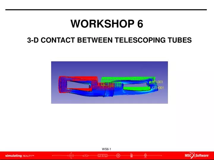
WORKSHOP 6 3-D CONTACT BETWEEN TELESCOPING TUBES
Model Description: • This ensemble represents two telescoping, cutout cylindrical pieces; the outer one fixed to a wall; the inner one fixed to a rigid surface that act as a driver; the driver rotates about a horizontal axis at the center of the cylinder on the wall, carrying the glued section of the inner piece. Contact occurs between the tubes. Rigid, Moving “Driver” Surface (Glued to inner Tube) Rigid, Fixed “Wall” Surface (Glued to Outer Tube) 3-D Deformable-to-Deformable Contact
Objectives: • Resolving a 3-D deformable body contact problem. • Required: • An Nastran bdf file named Tube_mesh.bdf in your working directory. (It should be provided together with this training material.) Important Note: The solution time for this exercise is approximately 15 minutes on a PC with a 1.1 GHz processor and 1 GB of ram. You should plan your work to allow for this delay.
Exercise Overview: • Import mesh from a Nastran bdf File. • Create two surfaces at opposite ends of the tubes; one to represent the rigid wall (to which the outer tube is to be glued); the other to represent the rigid driver (glued to the inner tube). • Define all four contact bodies (two deformable bodies and one rigid body). • Setup analysis with appropriate options as advised for job to converge. • Run and monitor analysis. • Import and post-process results.
Step 1. Open a New Database a b Open a new database , Structures Workspace. • Launch SimXpert. • Select Structures.
a b c d f e Step 2. Set Unit Set the units to English. • Select Tools / Options • Select Units Manager. • Click Standard Units. • Select the line containing English Units (in, lb, s…) • Click OK • Click Apply.
a b c d d Step 3. Set “Create a Individual Part for each Nastran Property” Set “When import a Nastran input file, create a individual part for each property. • Select General / Input/Output / Nastran Structures diaglog. • Switch off Reduce Parts option in Import area • Click Apply. • Click OK
Step 4. Import the Mesh a b c Import the required Mesh. • Select File / Import / Nastran • Select Tube_mesh.bdf as the File name. • Click 開啟.
Step 5. Create a New Part a b Create a New part • On Geometry tab, select Create Part from the Constraint group. • Enter Title as Rigid_1. • Click OK. c
d i b c g h f j a Step 6. Create a Geometric Surface Create a geometric surface by defining its four vertices. • Click on Filler in theSurface group • Uncheck Using Curves. • Click in the Entities text box. • Select Specify XYZ coordinates from the Pick Filters toolbar. • Enter -2.5 -2.5 0 then click OK. • Enter 2.5 -2.5 0 , click OK • Enter 2.5 2.5 0, click OK • Enter -2.5 2.5 0, click OK then Cancel. • Click OK on the Filler form. • Click Fill on the View Manipulation toolbar. e
Step 7. Create a New Part a b Create a New part • On Geometry tab, select Create Part from the Constraint group. • Enter Title as Rigid_2. • Click OK. c
d f i b c g h d j a Step 8. Create a Geometric Surface Create a geometric surface by defining its four vertices. • Click on Filler in theSurface group • Uncheck Using Curves. • Click in the Entities text box. • Select Specify XYZ coordinates from the Pick Filters toolbar. • Enter -2.5 -2.5 27,then click OK. • Enter 2.5 -2.5 27, click OK • Enter 2.5 2.5 27, click OK • Enter -2.5 2.5 27, click OK then Cancel. • Click OK on the Filler form. • Click Fill on the View Manipulation toolbar. e
Step 9. Define the Deformable Contact Body - Outer a Create contact body for pipe mesh • On LBC’s tab, select Contact \ Deformable Body (Structural) • Enter Outer as Name • Click Pick Entities field • Choose PSOLID_1_Tube_Mesh.bdf from Model Browser • Enter 0.1 as Friction Coefficient • Click Apply b c e f d d
Step 10. Define the Deformable Contact Body - Inner Create contact body for pipe mesh • Enter Inner as Name • Click Pick Entities field • Choose PSOLID_2_Tube_Mesh.bdf from Model Browser • Enter 0.1 as Friction Coefficient • Click OK a b d e c c
Step 11. Define the Rigid Contact Body – Rigid_Outer a Create the rigid contact object. • On LBC’s tab, select Contact \ Rigid Body (Structural) • Enter Rigid_Outer as the Name. • Click Pick Entities field • keep only Pick Surfaces optionfrom Pick Filters toolbar • Select the surface as the graph below • Select Body Tab • Check on ReverseInward Normals Option • Click Apply d b c f g e h
Step 11. Define the Rigid Contact Body – Rigid_Inner Create the rigid contact object. • Enter Rigid_Inner as the New Set Name. • Click Pick Entities field • keep only Pick Surfaces optionfrom Pick Filters toolbar • Select the surface as the graph below • Select Motion Tab • Enter0.0872665 as Angular Velocity (Rad/s) • Choose the node in the middle of the right side as figure shown • Enter Rotation Axis as X:-1 Y:0 Z:0 • Select Body Tab • Check off ReverseInward Normals Option • Click OK c a b e f g h k d i j
Step 12. Create Contact Table a Create Contact Table • On LBC’s tab, select Contact \ Table • Change the Contact Table as the figure shown • Click OK b c
Step 13. Create the Analysis Job Setup and launch the Analysis. • Right-click FileSet and select Create new Nastran Job. • Enter Telescope as the Job Name. • Solution Type: Implicit Nonlinear Analysis (SOL600). • Click OK a b c d
Step 14. Define Contact Parameters Setup the Analysis Parameter • Click right mouse button, Simulation / Telescope / Solver Control / Properties • Select ContactControlParameters dialog • Use vertical slide bar to move the dialog to Friction Parameters area • Choose Coulomb Type and Nodal Force Method • Enter Relative Sliding Velocity as 0.1 • Click Apply a b d e c f
Step 15. Setup Analysis Parameters Setup the Analysis Parameter • Click right mouse button, Simulation / Telescope / LoadCases / DefaultLoadCase / Properties • Select SOL600SubcaseNonlinearGeomParameter dialog • Switch Nonlinear Geometric Effects option to Large Displacement/Large Strains • Click Apply • Click Close a b c d e
Step 16. Select Contact Table Select Contact Table. • Right click on Simulations / Telescope / Load Cases / DefaultLoadCase / Select BCTABLE • Click BCTABLE_1 from Model Browser / Contact • Click OK. b a
Step 17. Run this job Run this job • Open Model Browser, click right mouse button at Telescope,select Run. a
Step 18. Attach the result file Read (Attach) results. • Select File / New to open a new database • File / Attach Results / Result Entities • Click on Telescope.marc.t16 • Switch Attach Options to Both • Click OK. c a d b e
Step 19. Plot the Deformation Results a c b d e Plot the deformation & stress results. • On the Results tab, select Deformation • Result Cases: select the Increment with Time=1.0 • Result type: Displacement, Translation • Click Display setting tab, change Deformed display scaling to “True :1”. • Choose Update
Step 20. Plot the Stress Results a d c b Plot the deformation & stress results. • Plot type: Fringe • Result Cases: select the Increment with Time=1.0 • Result type: Stress, Cauchy Equivalent • Choose Update