Download

1 / 29
290 likes | 430 Views
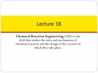
MA557/MA578/CS557 Lecture 16. Spring 2003 Prof. Tim Warburton timwar@math.unm.edu. Time Stepping Stability. Recall the Jameson-Shmidt-Turkel varient of the Runge-Kutta time integator:. Iterator.

E N D
MA557/MA578/CS557Lecture 16 Spring 2003 Prof. Tim Warburton timwar@math.unm.edu
Time Stepping Stability • Recall the Jameson-Shmidt-Turkel varient of the Runge-Kutta time integator:
Iterator • Recall the JST Runge-Kutta scheme unrolls to exactly discretize the first s+1 terms in the Taylor series (evaluated at t=n*dt):
Iterator cont • The iterator proves to be: • For the advection equations, we then replace the d/dt with a numerically discretization of the spatial derivative operator. • Suppose we diagonalize the spatial operator – i.e. we have created a number of decoupled (i.e. independent) iteration relationships. We will now consider one such iterator
Stability of Iteration • A sufficient condition for stability is that the L operator: • Is a contraction mapping (i.e. ||Lu||<= ||u||) • We seek the region of stability of L by looking for extremal curves where the inequality is an equality. Since the L operator is a scalar we look for curves in the complex plain where:
Computing the Stability Region • Let’s look at the stability of the first order J-S-T scheme: • We look for the solution of : • Solution:
Notes on the Stability Only onepoint on the imaginary axis is in thestability region Interior ofcircle is the Stable region
General Order Case (RK-s) • To find the stability curve(s) as a function of theta, we need to find the roots of the s+1 order polynomial: Matlab code: 3-6) build coefficients 8-9) loop over theta 10) Set coefficient of constant term 13) Find roots of polynomial 15) Plot roots
Stability Regions For s=1,2,3,4 • Note how the stability region grows in size. • This means that a fixed alpha, dt can be made larger if s is increased. • However, this is not strictly true if alpha lies near the extremal theta for the schemes (see theta = -1).
More Stability Notes • We zoom in: For the scheme to be stablefor an alpha dipping into theright half plane, the RK schememust be applying a certainamount of dissipation..
Class Exercise • Download the tstability script fromhttp://www.math.unm.edu/~timwar/MA578S03/MatlabScripts/tstability.m • Plot the stability regions up to s=8 • Identify which choices of s are likely to be most efficient (this will certainly depend on the range of dt*alpha
Time Step Restriction • So next we need to determine a bound on the eigenvalues (i.e. the spectral radius) of the spatial operator for the DG advection scheme. • Recall the upwind DG scheme:
Eigenvalue Bound • For the periodic case we already know that the real right hand side operator has negative real parts (non-increasing energy property): • Note we used the two inverse-inequalities we derived previously. • C1, C2 and C3 are independent of h (i.e. dx) and p
Finally: • We can now bound the eigenspectrum • And the real part of all the eigenvalues is non-positive. • So we know from the J-S-T stability analysis that it is sufficient for the semi circle defined by: to lie in the stability region of J-S-T scheme. • i.e. approx. for a given h,p,s choose dt such that:
Note From the class exercise and looking at the stability regions for J-S-T you should realize that the s dependence is dubious!!.The stability regions grow differentially in different directions – so watch out.
Example Eigenspectrum Sparsity pattern of operator Matlab script to construct upwind DG advection operator Distribution of eigenvaluesof upwind DG advection op.
Quick Discussion The script for building the operator is at: http://www.math.unm.edu/~timwar/MA578S03/MatlabScripts/umADEIGSwhole.m Let’s discuss dt issue.
Advection-Diffusion Equation • We now generalize the advection equation to include possible diffusion effects. • Examples of diffusion driven processes ??
Advection-Diffusion Equation • We consider the motion of a tracer solute in a fluid with mean velocity ubar. • We will denote the concentration of the tracer by C(x,t) • Not only is the tracer advected by the fluid’s mean velocity – it will also diffuse by random particle motion. • The advection-diffusion equation is:
Advection • The advection equation is as previously discussed: • i.e. the total tracer in a section of pipe is only changed by advection of the tracer through the ends of the section. • However, if the tracer particles are moving randomly then particles will randomly jump in and out of the section of pipe.
Diffusion • An underlying assumption of the ADE is that mechanical dispersion, like molecular diffusion, can be described by Fick’s first law: • where F is the mass flux of solute per unit area per unit time and D is the effective diffusion coefficient in a porous medium. • Fick.s law states that particle flux is directly proportional to the spatial concentration gradient. But it is not the spatial concentration gradient that causes particle movement, i.e. particles do not .push. each other (Crank, 1976). • Particles exhibit random motion on the molecular level. This random motion ensures that a tracer will diffuse, decreasing the concentration gradient (Crank, 1976). • Crank, J., 1976. The Mathematics of Diffusion. Oxford University Press, New York.
Diagram of Diffusion Model b a b Assume that each particle is jumping with a rate of R(delta) jumps per second which take it a distance of delta or more then there will be a number of jumps out of the left delta width ~= -R(delta)*0.5*delta*(C(b) + C(b-delta)) We count the number of jumps in from the right delta width ~= +R(delta)*0.5*delta*(C(b+delta)+C(b)) Summing:
Rough Derivation of Fickian Diffusion • Consider the x=b end of the section. We are going to “monitor” the random motions of a particle in and out of the region: • Assume that each particle is jumping with a rate of R jumps per second then there will be a flux of out of the b end (similar at the a end) • We apply tracer counting:
[ Note continuity assumptions ] We now recall that R is a function of delta and clearly R must be inversely proportional to delta. i.e. as the region we are monitoring shrinks to zero, the rate of random motions into and out of the control region increases… We denote and obtain:
Next Classes • Proof of stability • Estimate of time step restriction for J-S-T • Convergence for ADE • Discrete scheme