Download
1 / 123
1.25k likes | 1.44k Views
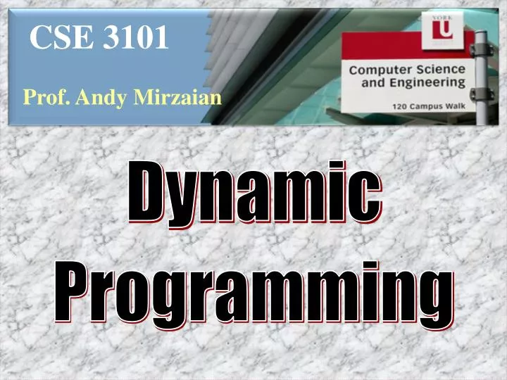
CSE 3101. Prof. Andy Mirzaian. Dynamic Programming. STUDY MATERIAL:. [CLRS] chapter 15 Lecture Note 9 Algorithmics Animation Workshop: Optimum Static Binary Search Tree. TOPICS. Recursion Tree Pruning by Memoization Recursive Back-Tracking Dynamic Programming

E N D
CSE 3101 Prof. Andy Mirzaian Dynamic Programming
STUDY MATERIAL: • [CLRS] chapter 15 • Lecture Note9 • Algorithmics Animation Workshop: • Optimum Static Binary Search Tree
TOPICS • Recursion Tree Pruning by Memoization • Recursive Back-Tracking • Dynamic Programming • Problems: • Fibonacci Numbers • Shortest Paths in a Layered Network • Weighted Event Scheduling • Knapsack • Longest Common Subsequence • Matrix Chain Multiplication • Optimum Static Binary Search Tree • Optimum Polygon Triangulation • More Graph Optimization problems considered later
Recursion Tree Pruning byMemoization Alice: We have done this sub-instance already, haven’t we? Bob: Did you take any memo of its solution? Let’s re-use that solution and save time by not re-doing it. Alice: That’s a great time saver, since we have many many repetitions of such sub-instances!
Re-occurring Sub-instances • In divide-&-conquer algorithms such as MergeSort, an instance is typically partitioned into “non-overlapping” sub-instances (e.g., two disjoint sub-arrays). That results in the following property: • For any two (sub) sub-instances, either one is a sub-instance of theother (a descendant in the recursion tree), or the two are disjoint & independent from each other. • We never encounter the same sub-instance again during the entire recursion. • If the sub-instances “overlap”, further down the recursion tree we may encounter repeated (sub) sub-instances that are in their “common intersection”. • Example 1: The Fibonacci Recursion tree (see next slide). • Example 2: Overlapping sub-arrays as sub-instances.
F(100) F(99) F(98) F(96) F(98) F(97) F(97) F(95) F(94) F(97) F(96) F(96) F(95) F(96) F(95) F(96) F(95) F(95) F(94) F(95) F(94) F(94) F(93) Fibonacci Recursion Tree AlgorithmF(n) ifn{0,1} then returnn return F(n-1) + F(n-2) end But only n+1 distinct sub-instances are ever called: F(0), F(1), …, F(n-2), F(n-1), F(n).Why is it taking time exponential in n?
F(n) F(n-1) F(n-2) F(n-2) F(n-3) F(n-3) F(n-4) F(n-4) F(n-5) F(2) F(n-3) F(1) F(0) Pruning by Memoization AlgorithmFib(n) for t 0 .. 1 do Memo[t] t for t 2 .. n do Memo[t] null § initialize Memo[0..n] tablereturn F(n) end FunctionF(n) § recursion structure kept if Memo[n] = null then Memo[n] F(n-1) + F(n-2) §memo feature added returnMemo[n] end Recursion tree evaluated in post-order. Now all right sub-trees are pruned. Instead of re-solving a sub-instance, fetch its solution from the memo table Memo[0..n]. T(n) = Q(n). Time-space trade off.
F(n) F(n-1) F(n-2) F(n-2) F(n-3) F(n-3) F(n-4) F(n-4) F(n-5) F(2) F(n-3) F(1) F(0) Memoization: Recursive vs Iterative AlgorithmFib(n)§ recursive top-down for t 0 .. 1 do Memo[t] t for t 2 .. n do Memo[t] null return F(n) end FunctionF(n) if Memo[n] = null then Memo[n] F(n-1) + F(n-2) returnMemo[n] end AlgorithmFib(n)§ iterative bottom-up (from smallest to largest) for t 0 .. 1 do Memo[t] t for t 2 .. n do Memo[t] Memo[t-1] + Memo[t-2] returnMemo[n] end
s u v CompactMemoization • We want compact memos to save both time and space. • Fibonacci case is simple; memoize a single number per instance. • What if the solution to a sub-instance is a more elaborate structure? • Examples: • Sub-instance solution is subarray A[i..j]: Just store (i,j), its first and last index. • Sub-matrix A[i..j][k..t]: Just store the 4 indices (i,j,k,t). • Solutions to sub-instances are sequences. Furthermore, any prefix of such a sequence is also a solution to some “smaller” sub-instance.Then, instead of memoizing the entire solution sequence, we can memoize its next-to-last (as well as first and last) elements. We can recover the entire solution á postiori by using the prefix property. • Single-source shortest paths. If the last edge on the shortest path SP(s,v) from vertex s to v is edge (u,v), then memo s,u,v (and path length) for the solution to that sub-instance. We can consult the solution to sub-instance SP(s,u) to find “its” last edge, and so on. Á postiori, working backwards, we can recover the entire sequence of vertices on the path from s to v.
RecursiveBack-Tracking Alice: I know my options for the first step. Can you show me the rest of the way? Bob: OK. For each first step option, I will show you the best way to finish the rest of the way. Alice: Thank you. Then I can choose the optionthat leads me to the overall best complete solution.
Solving Combinatorial Optimization Problems • Any combinatorial problem is a combinatorial optimization problem:For each solution (valid or not) assign an objective value: 1 if the solution is valid, 0 otherwise. Now ask for a solution that maximizes the objective value. Sorting: find a permutation of the input with minimum inversion count. • Greedy Method:Fast & simple, but has limited scope of applicability to obtain exact optimum solutions. • Exhaustive Search:A systematic brute-force method that explores the entire solution space. Wide range of applicability, but typically has exponential time complexity. • . . .
Solving COP by Recursive Back-Tracking • Recursive Back-Tracking (RecBT): • Divide the solution space for a given instance into a number of sub-spaces. • These sub-spaces must themselves correspond to one or a group of sub- instances of the same structure as the main instance. • Requirement: the optimum sub-structure property. • Recursively find the optimum solution to the sub-instances corresponding to each sub-space. • Pick the best among the resulting sub-space solutions. This best of the best is the overall optimum structure solution for the main instance. NOTE: Divide-&-Conquer and Recursive BT vastly differ on what they divide. D&C divides an instance in one fixed way into a number of sub-instances. RecBT divides the solution space into sub-spaces. • This is done based on one or more sub-division options. • Each option corresponds to one of the said sub-spaces. • Each option generates one or more sub-instances whose complete solution corresponds to the solution within the corresponding sub-space.
RecBT Solution Sub-Spaces Take best of these best solutions within each solution subspace
RecBT Recursion Tree • How should we divide the entire solution space into sub-spaces, so that each sub-space corresponds to a (smaller) instance or a group of (smaller) instances of the same type as the main problem we are trying to solve? • The Recursion tree: • Its root corresponds to the main instance given. • There are two types of nodes: • Sub-instance nodes appear at even depths of the recursion tree, • Sub-division option nodes appear at odd depths of the recursion tree. • For a specific (sub-) instance node, we may have a number of options on how to further divide it into groups of (sub-) sub-instances. For each such option, we have a sub-division option node as a child. Each option node has a group of children, each of which is a sub-instance node. • The leaves of the tree correspond to base case instances. • Examples follow ……………………………………………………… P.T.O.
x1, x2, … , xm, … Instance level xm= 1 xm= 0 sub-division option level x1, x2, … , xm-1, … x1, x2, … , xm-1, … Instance level Example 1: RecBT Recursion Tree 0/1 binary decision on a sequence X = x1, x2, … , xm. A simple situation: each division option node generates a single sub-instance child.
x1, x2, … , xm, … xm = 1 xm = 0 x1, x2, … , xm-1, … x1, x2, … , xm-1, … Example 1:RecBTRecursion Tree 0/1 binary decision on a sequence X = x1, x2, … , xm. A simple situation: each division option node generates a single sub-instance child.
((X1 1 X2 ) 2 ((X3 3 X4 ) 4 X5)) (((X1 1 (X2 2 X3)) 3 (X4 4 X5)) 3 2 4 4 1 1 X5 3 X5 X1 2 X4 X1 X2 X3 X4 X2 X3 Example 2:RecBT Recursion Tree Find optimum full parenthesization of (X1 X2 … Xk Xk+1 … Xn), where is an associative binary operator and Xk’s are operands. First, let’s see what a feasible solution looks like:It can be viewed by the full parenthesization, or by its parse tree. (Note: parse tree recursion tree.)
(X1 1 … Xk k Xk+1 … n-1Xn) n-1 k 1 (X1 1 … k-1Xk) (Xk+1 k+1 … n-1Xn) Example 2:RecBTRecursion Tree Find optimum full parenthesization of (X1 1 X2 2 … Xk k Xk+1 … n-1 Xn). Decision: which of 1 , … , k , … , n-1 should be performed LAST, i.e, form the root of the parse tree? Induces n-1 top level sub-division option nodes.
a1 a2 a3 a4 a5 G: 8 7 4 3 4 2 1 8 2 2 a6= t s = a0 2 3 6 1 9 3 3 2 5 6 b1 b2 b3 b4 b5 Shortest s-t path in Layered Network Notation: • Layers 0..n in graph G. s = starting vertex at layer 0, t = terminal vertex at layer n.For now assume O(1) vertices per layer. • w(u,v) = weight (or length) of edge (u,v) in G. • SP(u,v) = shortest path in G from vertex u to v (as a sequence of vertices).CostSP(u,v) = cost (or length) of SP(u,v). • Example: SP(a1,b4) = a1, b2, a3, b4 CostSP(a1,b4) = w(a1,b2) + w(b2,a3) + w(a3,b4) = 1+3+2 = 6. • 3 algorithmic solutions: Recursive Back-Tracking without Pruning Recursive Back-Tracking with Memoized Pruning Iterative Memoized Algorithm
a1 a2 a3 a4 a5 G: 8 7 4 3 4 2 1 8 2 2 a6= t s = a0 2 3 6 1 9 3 3 2 5 6 b1 b2 b3 b4 b5 Shortest s-t path in Layered Network • Optimum sub-structure property: • Any sub-path of a shortest path is a shortest path. • More specifically, removing the last edge of a shortest path results in a prefix path with one less edge that is itself a shortest path. • Last edge on SP(s,t) is either (a5, t) or (b5, t).Option 1. (a5, t): The rest of SP(s, t) must be SP(s, a5).Option 2. (b5, t): The rest of SP(s, t) must be SP(s, b5). • SP(s, t) = best of { SP(s, a5), (a5, t) , SP(s, b5), (b5, t) }CostSP(s, t) = min{ CostSP(s, a5) + w(a5, t), CostSP(s, b5) + w(b5, t) } • All sub-instances are of the form SP(s, u), where u is any vertex of G.
v1 s u v2 vk s p(u) u Shortest s-t path in Layered Network • Short-hand notation:SP(u) = SP(s,u), for any vertex u of G. (Starting vertex is always s.)CostSP(u) = CostSP(s,u) • p(u) = predecessor of vertex u on the shortest path from s to u. • SP(u) = SP(p(u)), u by the optimum sub-structure property. FACT:SP(u) = SP(p(u)), u , where p(u) { v | (v,u) is an edge in G } p(u) =argminv { CostSP(v) + w(v,u) | (v,u) is an edge in G } CostSP(u) = min v { CostSP(v) + w(v,u) | (v,u) is an edge in G } = CostSP(p(u)) + w(p(u) ,u)
a1 a2 a3 a4 a5 G: 8 7 4 3 4 2 1 8 2 2 a6= t s = a0 2 3 6 1 9 3 3 2 5 6 b1 b2 b3 b4 b5 Recursive Back-Tracking without Pruning AlgorithmShortestPath(G, s, u) Pre-Cond: G = a weighted layered digraph, u = a vertex of G, s = source vertex. Post-Cond: output is SP(u), CostSP(u) ifu = sthenreturn s, 0 § base case §CostSP(u) = min v { CostSP(v) + w(v,u) | (v,u) is an edge in G } cost for each vertex vV(G) : (v,u)E(G)do prefixSP, prefixCost ShortestPath(G, s, v) ifcost > prefixCost + w(v,u)thencost prefixCost + w(v,u); SP prefixSP, u end-for return SP , cost end 2O(n) time.
a1 a2 a3 a4 a5 G: 8 7 4 3 4 2 1 8 2 2 a6= t s = a0 2 3 6 1 9 3 3 2 5 6 b1 b2 b3 b4 b5 SP , cost ShortestPath(G, s, t) Print SP 2O(n) time. O(n) time. Á PostioriPrint Shortest s-t Path
Recursive Back-Tracking with Memoized Pruning Memo[V(G)] = an array indexed by V(G).u V(G): Memo[u] = Memo.p[u] , Memo.CostSP[u] . AlgorithmShortestPath(G, s, t)§G = a layered graph … for each vertex u V(G) doMemo[u] nil, §Initialize memo table end-for Memo[s] nil, 0 § base case SP(G, s, t) § compute shortest pathsPrintSP(G, s, t) § print shortest s-t path end ProcedureSP(G, s, u) ifu = sthenreturn§ base casefor each vertex vV(G) : (v,u)E(G)doifMemo.CostSP[v] = thenSP(G, s, v) ifMemo.CostSP[u]>Memo.CostSP[v] + w(v,u)thenMemo.CostSP[u] Memo.CostSP[v] + w(v,u);Memo.p[u] v end-for end
Recursive Back-Tracking with Memoized Pruning Memo[V(G)] = an array indexed by V(G).u V(G): Memo[u] = Memo.p[u] , Memo.CostSP[u] . AlgorithmShortestPath(G, s, t)§G = a layered graph … for each vertex u V(G) doMemo[u] nil, §Initialize memo table end-for Memo[s] nil, 0 § base case SP(G, s, t) § compute shortest pathsPrintSP(G, s, t) § print shortest s-t path end Q(n) time ProcedurePrintSP(G, s, u) Pre-Cond: G = a weighted layered digraph, u = a vertex of G, s = source vertex. Post-Cond: output is SP(u), the shortest path from s to u in G. ifu = nilthenreturn§ base case PrintSP(G, s, Memo.p[u]) print u end
IterativeMemoized Algorithm The closer the layer of u is to s, the “lower” the sub-instance is in the recursion tree, the earlier we need to solve it iteratively “bottom-up”.Solutions to larger sub-instances depend on the smaller ones. AlgorithmShortestPath(G, s, t)§G = a layered graph … for each vertex u V(G) do §Initialize memo table p[u], Cost[u] nil, Cost[s] 0forlayer 1 .. ndo§ in a reverse order of dependency for each vertex u in layerdofor each vertex vV(G) : (v,u)E(G)doifCost[u]> Cost[v] + w(v,u)thenCost[u] Cost[v] + w(v,u);p[u] vPrintSP(G, t) end Q(n) time ProcedurePrintSP(G, u)§ O(n) timeifu = nilthenreturn§ base case PrintSP(G, p[u]); print u end
a1 a2 a3 a4 a5 G: 8 7 4 3 4 2 1 8 2 2 a6 = t s = a0 2 3 6 1 9 3 3 2 5 6 b1 b2 b3 b4 b5 An Example Run AlgorithmShortestPath(G, s, t)§G = a layered graph … for each vertex u V(G) do §Initialize memo table p[u], Cost[u] nil, Cost[s] 0forlayer 1 .. ndo§ in a reverse order of dependencyfor each vertex u in layerdofor each vertex vV(G) : (v,u)E(G)doifCost[u] > Cost[v] + w(v,u)thenCost[u] Cost[v] + w(v,u);p[u] vPrintSP(G, t) end Q(n) time 2 10 6 10 9 13 9 3 5 8 12
Path(s,t) = Path(s,u) , Path(u,t) (u is an intermediate vertex on the path) Path(u,t) Path(s,u) t s u Caution! The Optimum Sub-Structure Property (OSSP) is vital. Example: Optimum simple paths in a given positively weighted graph G. • LongestSimple Paths. (simplicity excludes cycles on the path) • Shortest Simple Paths. The 1st one does NOT have the OSSP, but the 2nd does! Path(s,t) is longest s-t path does NOT imply that Path(s,u) is longest s-u path, nor that Path(u,t) is longest u-t path. Path(s,t) is shortest s-t path does imply that Path(s,u) is shortest s-u path, and that Path(u,t) is shortest u-t path. Explain the discrepancy! In the 1st case, sub-instances interfere with each other (not independent).
u 2 6 3 2 s t 7 8 v s, u, v, t is the longest simple s-t path, but the sub-path s, u is not the longest simple s-u path! Longest simple s-u path is s, v, u.Replacing s, u by s, v, u in s, u, v, t results in thenon-simple path s, v, u, v, t. WITHOUT CYCLES IN G, THIS WON’T HAPPEN! Caution!
WEIGHTEDEVENT SCHEDULING A banquet hall manager has received a list of reservation requests for the exclusive use of her hall for specified time intervals. Each reservation also indicates how much they are willing to pay. She wishes to make the most profit by granting a number of reservation requests that have no time overlap conflicts. Help her select the maximum profitable conflict free time intervals.
time w2=6 w7= 10 w9= 2 w4= 7 w8= 5 w1= 2 w3= 3 w6= 4 w10= 5 w5= 8 Weighted Event Scheduling Input: A set S = { I1, I2, ···, In} of n weighted event time-intervals Ik = sk , fk, wk, k =1..n, where sk < fk are start and finishing times, and wk > 0 is the weight of Ik. Feasible Solutions: Any subset C S with no overlapping pair of intervals. Objective Value:W(C) = sum of the weights of intervals in C. Goal: Output a feasible solution C with maximum W(C). Reminder:We studied a greedy solution for the un-weighted case, i.e., wk = 1, for k=1..n. Example: S = the weighted intervals shown below,C = the set of blue intervals (happens to be the unique optimum), W(C) = 6 + 8 + 5 = 19. (Note: the greedy strategy fails here.)
Implicit reduction to a special graph path problem: fk sm 0 fk sm Ik = sk , fk , wk ignore transitive edges Find longest path from f- to s+ : s2 f2 s7 f7 s9 f9 w2 sk fk w7 w9 wk s4 f4 f8 w1 w8 w4 s8 f- s+ time s1 f1 w2=6 w7= 10 w9= 2 f6 w4= 7 w8= 5 w1= 2 s3 w3 w6 f3 s6 w10 w3= 3 w5 w6= 4 w10= 5 w5= 8 s10 f10 s5 f5
sk fk sm fm 0 wm f- p(m) = k W(m) = W(k)+wm Longest path in the graph The digraph is acyclic OSSP holds for longest paths. LP(u) = Longest path from source to node u. W(u) = weight (or length) of LP(u) [ W(f- ) = 0 ] p(u) = predecessor of node u on LP(u). FACT: LP(u) = LP(p(u)), u , where p(sm) = argmaxk { W(fk) | (fk, sm) is an edge in G } W(sm) = W(p(sm)) = max k { W(fk) | (fk, sm) is an edge in G } W(fm) = W(sm) + wm Memo(Im) = p(m) ,W(m) = p(sm) ,W(fm) . Scan Order: Sort starting & finishing times, and scan nodes in that order (as if you were working with a layered graph).
AlgorithmOptWeightEventSchedule( S = {Ik = sk , fk, wk | k =1 ..n } ) Pre-Cond: S is an instance of the weighted event scheduling problem. Post-Cond: The optimum schedule C is returned. EventNodes {sk , k | k =1 ..n } {fk , k | k =1 ..n } Sort EventNodes in ascending order of the first componentpnode , pW nil , 0 § memo of opt path ending just before the next nodefor each t , k EventNodes, in sorted order doift = skthenp(k) pnode ; W(k)pW + wk else §t = fkifpW < W(k)thenpnode , pW k , W(k) end-for C ; k pnodewhilek nil do C C {Ik}; k p(k) return C end O(n log n) time
Dynamic Programming Alice: Now I see that I can save a great deal of time by using some extra amount of memory space to take memos. Using that, I can avoid reworking on repeated sub-instances. Bob: (1) Make sure the VIP herself, Mrs. OSSP, is present!OSSP is needed to express solutions of larger sub-instances in terms of smaller ones.(2) You can choose recursive top-down or iterative bottom up. (3) If you choose iteration, solve and memoize all possible sub-instances in reverse order of dependency. (4) How many distinct sub-instances do you have, polynomial or exponential?That determines the memo table size and affects time & space complexity.
Dynamic Programming = Recursive Back-Tracking + OSSP +Memoized Pruning . Dynamic Programming Design Steps: • Think about the recursion tree structure, its post-order evaluation, & how you will sub-divide an instance into (smaller) immediate sub-instances using sub-division option nodes. Identify base cases. • Make sure this sub-division into sub-instances satisfies the OSSP. • Determine the set of all possible distinct sub-instances that would be recursively generated in the recursion tree. (Moderate over-shooting is OK.) Make sure this set is closed under the sub-division in step 1. • Using OSSP, develop the DP Recurrence Formula that expresses the memo of the optimum solution of each (sub-)instance in terms of the memos of optimum solutions to its (smaller) immediate (sub-)sub-instances. This formula has to be general enough to be valid for each sub-instance in the set of sub-instances determined in step 3. Express base cases by some direct method. • Starting from the base cases, iteratively fill in the memo table in reverse order of dependency using the recurrence from step 4. • Ápostiori, use the memo table to recover & reconstruct the optimum solution to the given main instance. • Keep an eye on time & space efficiency.
PROBLEMS • Fibonacci Numbers (done) • Shortest Paths in a Layered Network (done) • Weighted Event Scheduling (done) • The Knapsack Problem • Longest Common Subsequence • Matrix Chain Multiplication • Optimum Static Binary Search Tree • Optimum Polygon Triangulation • More graph problems later.
THE KNAPSACK PROBLEM • Optimum subset of items that fit in the knapsack. • Optimum subset of profitable investments with limited budget.
The Knapsack Problem Input: Items 1..n with weights w1, w2, … , wn and values v1, v2, … , vn, and knapsack weight capacity W (all positive integers). Feasible Solutions: Any subset S of the items (to be placed in the knapsack) whose total weight does not exceed the knapsack capacity W. Objective value: V(S) = SkSvk. Goal: Output a feasible solution S with maximum objective value V(S). Example: Greedy 1: Max vk first: S1 = {1}, V(S1) = 28. Greedy 2: Max vk / wk first: S2 = {3, 5}, V(S2) = 24 + 5 = 29. Optimum: SOPT = {2, 5}, V(SOPT) = 27 + 5 = 32.
level n [1..n], W xn =1 xn =0 level n-1 [1..n-1], W [1..n-1], W -wn xn-1 =0 xn-1 =0 xn-1 =1 xn-1 =1 level n-2 [1..n-2], W -wn-wn-1 [1..n-2], W -wn [1..n-2], W -wn-1 [1..n-2], W level k [1..k], W’ xk =0 xk =1 [1..k-1], W’–wk [1..k-1], W’ , … , … base level (boundary condition) Think about the recursion tree structure, its post-order evaluation, & how you will sub-divide an instance into (smaller) immediate sub-instances using sub-division option nodes. Identify base cases. Dynamic Programming Design Step 1: • Root of the recursion tree corresponds to the main instance, involving all n items. • Each node at the kth level of the recursion tree corresponds to a sub-instance concerning the subset of the items [1 .. k ]. (Objective value & Knapsack capacity … later!) • At a node on the kth level, we make a 0/1 decision on the kth variable xk. • Each node at that level has 2-way branching: • 1-branch: include item k in the solution of that sub-instance, • 0-branch: exclude item k in the solution of that sub-instance.
[1..k], W’ xk =0 xk =1 [1..k-1], W’–wk [1..k-1], W’ Make sure this sub-division into sub-instances satisfies the OSSP. Dynamic Programming Design Step 2: • OSSP is satisfied: Consider an arbitrary sub-instance ([1..k], v1, v2, … , vk , w1, w2, … , wk , W’) at level k. • Suppose x1, x2, … , xk OPT ([1..k], v1, v2, … , vk , w1, w2, … , wk , W’) • Case 0) xk = 0. Then,x1, x2, …, xk-1 OPT ([1..k-1], v1, v2, … , vk-1 , w1, w2, … , wk-1 , W’).Case 1) xk = 1. Then,x1, x2, …, xk-1 OPT ([1..k-1], v1, v2, … , vk-1 , w1, w2, … , wk-1 , W’ – wk ). • Why? Because if they were not, by cut-&-paste, we could replace them with a better feasible solution x1, x2, …, xk-1 forthe respective knapsack capacity. But that would contradict theoptimality of x1, x2, …, xk-1 , xk for the bigger instance.
Determine the set of all possible distinct sub-instances that would be recursively generated in the recursion tree. (Moderate over-shooting is OK.) Make sure this set is closed under the sub-division in step 1. Dynamic Programming Design Step 3: • Any sub-instance that could possibly be generated in the recursion tree has the form: ([1..k], v1, v2, … , vk , w1, w2, … , wk , W’) for some k = 0..n, & some integer W’ W. • If W’ < 0, the corresponding sub-solution has conflict and will not result in any feasible solution. So, we prune the recursion sub-tree at that point immediately. • Beyond this, we won’t further pin-point which specific values of W’ will show up.So, we consider any W’ in the integer range 0..W.This is an over-shoot we will live with. • So, all the sub-instances are of the form:([1..k], v1, v2, … , vk , w1, w2, … , wk , W’) for k = 0..n, & W’ = 0 .. W. • k = 0 or W’ = 0 form the boundary cases. Why?
Using OSSP, develop the DP Recurrence Formula that expresses the memo of the optimum solution of each (sub-)instance in terms of the memos of optimum solutions to its (smaller) immediate (sub-)sub-instances. This formula has to be general enough to be valid for each sub-instance in the set of sub-instances determined in step 3. Express base cases by some direct method. Dynamic Programming Design Step 4: VOPT(k, W’) = the optimum solution value for the instance ([1..k], v1, v2, … , vk, w1, w2, … , wk , W’), k = 0..n, W’ = 0..W. Memo table: (n+1)(W+1) matrix VOPT[ 0..n, 0..W].
Boundary condition: row 0 and column 0 0……W’–wk……...W’………. W 0 . . k-1 k . . n the 2 arrows show dependence VOPT : Memo table: (n+1)(W+1) matrix VOPT[ 0..n, 0..W].
Starting from the base cases, iteratively fill in the memo table in reverse order of dependency using the recurrence from step 4. Dynamic Programming Design Step 5: AlgorithmKnapsack( v1, v2, … , vn, w1, w2, … , wn , W ) Pre-Cond: input is a valid instance of the Knapsack Problem Post-Cond: optimum 0/1 knapsack solution x1, x2, … , xn is returnedfor W’ 0 .. W do VOPT[0,W’] 0§boundary cases firstfor k 0 .. n do VOPT[k,0] 0§boundary cases firstfork 1 .. ndo§ in a reverse order of dependency for W’ 1 .. W doVOPT[k,W’] VOPT[k-1,W’] ifwk W’then ifVOPT[k,W’] < vk + VOPT[k-1, W’ – wk] thenVOPT[k,W’] vk + VOPT[k-1, W’ – wk] end-for end-for returnOptSol(v1, v2, … , vn, w1, w2, … , wn , W, VOPT) end Q(nW) time & space
0……...……………………… W 0 . . . . . . n VOPT : Ápostiori, use the memo table to recover & reconstruct the optimum solution to the given main instance. Dynamic Programming Design Step 6: AlgorithmOptSol(v1, v2, … , vn, w1, w2, … , wn , W, VOPT) W’ W fork n downto 1do§ work backwards on the memo table ifVOPT[k,W’] = VOPT[k-1,W’] then xk 0elsexk 1; W’ W’ – wk end-for return (x1, x2, … , xn) end Q(n) time
Keep an eye on time & space efficiency. Dynamic Programming Design Step 7: Time = Q(nW), Space = Q(nW). This is not polynomial but exponential. Input number W requires log W bits. We don’t know of any polynomial time algorithm for the 0/1 Knapsack Problem.We shall later see that 01KP is one of the so called NP-hard problems. What other options do we have? • Find good approximations to the optimum solution (done in CSE 4101). • Consider relaxing the feasibility constraints to allow fractional valuesfor the variables (not just 0/1 values). GREEDY 2 (already discussed) is correct for the fractional case! ………………………..………………………………………………………. P.T.O.