Download
1 / 62
620 likes | 630 Views
Early models of an expanding Universe. Paramita Barai Astr 8900 : Astronomy Seminar 5th Nov, 2003. Contents. Introduction Discuss papers : 1922 : Friedmann 1927 : Lema î tre 1932 : Einstein & De Sitter Present cosmological picture Some results SN project, WMAP, SDSS.

E N D
Early models of an expanding Universe Paramita Barai Astr 8900 : Astronomy Seminar 5th Nov, 2003
Contents • Introduction • Discuss papers : • 1922 : Friedmann • 1927 : Lemaître • 1932 : Einstein & De Sitter • Present cosmological picture • Some results • SN project, WMAP, SDSS
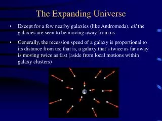
Cosmological foundations • Cosmological principle • Universe is Homogeneous & Isotropic on large scales (> 100Mpc) • Universe (space itself) expanding, dD/dt ~ D (Hubble Law) • Universe expanded from a very dense, hot initial state (Big Bang) • Expansion of universe – mass & energy content – explained by laws of GTR Dynamics of universe • Structure formation in small scales (<10-100 Mpc) by gravitational self organization • WHAT IS THE GEOMETRY OF OUR UNIVERSE, & IT’S CONSEQUENCES ??
Cosmological parameters • R – Scale factor of Universe • Critical density , C – density to make universe flat (it just stops expanding) • Density parameter, = / C • H = Hubble constant = v / r • = Cosmological Constant (still speculative!!) • Dark Energy • Repulsive force, opposing gravity
Curvature of space • Positive curvature – Closed – contract in future • > C • > 1 • Zero curvature – Flat – stop expansion in future & stationary • = C • = 1 • Negative curvature – Open – expand forever • < C • < 1
Timeline • 1905 – Einstein’s STR, 1915 – GTR • 1917 – Einstein & De Sitter static cosmological models with • 1922 – Friedmann • First non-static model • Universe contracts / expands (with ) • 1927 – Lemaître – expanding universe • 1930 – Hubble: expanding universe, Einstein drops (“biggest blunder”) • 1932 – Einstein & de Sitter • Expanding universe of zero curvature
Timeline – cont’d… • 1948 – Particle theory (QED) predicts non zero vacuum energy , but QED = 10120other • 1965 – CMBR • Early 1980’s: LUM << C Open universe • 1980’s – • Inflation theory Flat universe (TOT = 1) • Dark matter • 1990’s - LUM~ 0.02-0.04, DARK ~ 0.2-0.4, REST= ? • 1998 – Accelerating universe • Present model – universe very near to flat (with matter and vacuum energy)
Matter density = 0 Advantage : Explains naturally observed radial receding velocities of extra galactic objects From consequence of gravitational field Without assuming we are at special position Parameters c = velocity of light = Cosmological constant = Density of universe Two first models of universe:De Sitter
Non zero matter density Relation between density & radius of universe masses much greater than known in universe at that time Can’t explain receding motion of galaxies Advantage Explains existence of matter Parameters = Einstein constant = 1.8710-27 (cgs) Einstein universe
Curvature of space Aleksandr Friedman Zeitschrift fur Physik 10, 377-386, 1922
Summary • First non static model of universe • Work immediately not noticed, but found important later … • R independent of t : • Stationary worlds of Einstein & de Sitter • R depends on time only : • Monotonically expanding world • Periodically oscillating world • depending on chosen
Goal of the paper • Derive the worlds of Einstein & de Sitter from more general considerations
Assumptions of 1st class • Same as Einstein & de Sitter • Gravitational potentials obey Einstein field equations with cosmological term • Matter is at relative rest
Assumptions of 2nd class • Space curvature is constant wrt 3 space coordinates; but depends on time • Metric coefficients: g14, g24, g34 = 0, suitable choice of time coordinate
R(x4) = 0 M = M0 = constant Cylindrical world Einstein’s results M = (A0x4+B0) cos x1 Transform x4 De Sitter spherical world (M=cos x1) Solutions: Einstein & de Sitter worlds as special cases Stationary world
R(x4) 0 M = M(x4) But – suitable x4 – M = 1 Non stationary world
R ( > 0 ) Increases with t Initial value, R = R0 (>0) at t = t0 R = 0, at t = t t = Time since creation of world Monotonic world of first kind > 4c2/9A2
Time since creation of world, t R increases with t Initial R = x0 x0 & x0 are roots of equation: A-x+(x3/3c2) = 0 Monotonic world of second kind 0 < < 4c2/9A2
R – periodic function of t World Period = t Periodic World t if Small , approximate - < < 0
Possible universes of Friedmann • Monotonic worlds • > 4c2/9A2 • First kind • 0 < < 4c2/9A2 • Second kind • Periodic universe • - < < 0
Conclusions • Insufficient data to conclude which world our universe is … • Cosmological constant, is undetermined … • If = 0, M = 5 1021 M • Then, world period = 10 billion yrs • But this only illustrates calculation
A Homogeneous universe of Constant Mass & Increasing Radius accounting for the Radial Velocity of Extra – Galactic NebulaeAbbe Georges Lemaître • Annales de la Société scientifique de Bruxelles, A47, 49, 1927 • English translation in MNRAS, 91, 483-490, 1931
Summary • Dilemma between de Sitter & Einstein world models • Intermediate solution – advantages of both • R = R(t) • R(t) as t • Similar differential equation of R(t) as Friedmann
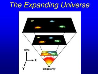
Summary cont’d.… • Accounted the following: • Conservation of energy • Matter density • Radiation pressure • Role in early stages of expansion of universe • First idea: • Recession velocities of galaxies are results of expansion of universe • Universe expanding from initial singularity, the ‘primeval atom’
Intermediate model • Solution intermediate to Einstein & De Sitter worlds • Both material content & explaining recession of galaxies • Look for Einstein universe • Radius varying with time arbitrarily
Universe ~ Sparsely dense gas Molecules ~ galaxies Uniformly distributed Density – uniform in space, time variable Ignore local condensation Internal stresses ~ Pressure p = (2/3) K.E. Negligible w.r.t energy of matter Radiation pressure of E.M. wave Weak Evenly distributed Keep p in general eqn For astronomical applications, p = 0 Assumptions of model
Field equations : conservation of energy • Einstein field equations • = Cosmological Constant (unknown) • = Einstein Constant • Total energy change + Work done by radiation pressure in the expanding universe = 0
= Total density = Matter density = - 3p Mass, M = V = constant = constant = integration constant Equations: Universe of constant mass
De Sitter world = 0 = 0 Einstein world = 0 R = constant Existing solutions
R0 = Initial radius of universe (from which expanding) R = Lemaître distance scale at time t RE = Einstein distance scale at t For = 0 & = 2R0 Lemaître solution
Cosmological Redshift • R1, R2 = Radius of Universe at times of emission & observation of light • Apparent Doppler effect • If nearby source, r = distance of source
Einstein radius of universe: by Hubble from mean density RE = 2.7 1010 pc If R0 from radial velocities of galaxies R from R3 = RE2 R0 From data R/R = 0.6810-27 cm-1 R0/R = 0.0465 R = 0.215RE = 6 109 pc R0 = 2.7 108 pc = 9 108 LY Values Calculated
Mass of universe – constant Radius of universe – increases from R0 (t = -) Galaxies recede as effect of expansion of universe Advantage of both Einstein & de Sitter solutions Conclusions
Expanding space Possible universe of Lemaître
100 Mt. Wilson telescope range: 5 107 pc = R / 200 Doppler effect – 3000 km/s Visible spectrum displaced to IR Why universe expands? Radiation pressure does work during expansion expansion set up by radiation itself Limitations & Further scopes
On the relation between Expansion & mean density of universeAlbert Einstein& Wilhelm de sitter(Proceedings of the National Academy of Sciences 18, 213 – 214, 1932)
Summary • After Hubble discovered expansion of universe: Einstein & de Sitter withdrew • Expanding universe – without space curvature • If matter = C= 3H2/(8G) • Euclidean geometry • Flat, infinite universe • Using H0 ~ 10 H0 today • G(optically visible galaxies) ~ C Flat space
Motivation • Observational data for curvature • Mean density • Expansion Universe – non static • Can’t find curvature sign or value • If can explain observation without curvature ??
to explain finite mean density in static universe Dynamic universe – without = 0 Line element: R = R(t) Neglect pressure (p) Field equation => 2 differential eqns Zero curvature
From observation H - coefficient of expansion - mean density From H = 500 km sec-1 Mpc-1 or, RB = 2 1027 cm Get RA = 1.63 1027 cm = 4 10-28 g cm-3 Coincide exactly with theoretical upper limit of density for Flat space Solutions
H – depends on measured redshifts Density – depends on assumed masses of galaxies & distance scale Extragalactic distances Uncertain H2 / or RA2/RB2 ~ /M = Side of a cube containing 1 galaxy = 106 LY M = average galaxy mass = 2 1011 M ~ close to Dr. Oort’s estimate of milky way mass Confidence limit of solution
- higher limit Correct magnitude order Possible to describe universe without curvature of 3-D space However, curvature is determinable More precise data Fix curvature sign Get curvature value Conclusions
Present status of cosmological model • Search for cosmological parameters determining dynamics of universe: • Hubble constant, H0 • TOT = M + + K • M = M/C • Matter (visible+dark) • = / 3H02 • Vacuum energy • K = -k / R02H02 • Curvature term • If flat k = 0
H0 Hubble key project WMAP H0 = (71 3) km/s/Mpc M Cluster velocity dispersion Weak gravitational lens effect visible ~ 0.02 – 0.04 dark ~ 0.25 M ~ 0.3 Current values
• Energy density of vacuum • Discrepancy of > 120 orders of magnitude with theory • ~ 0.7 • SN Type Ia • WMAP • Age of universe: • t0 = 13.7 G yr
SN Type Ia • Giant star accreting onto white dwarf • Standard candle • Compare observed luminosity with predicted • Far off SN fainter than expected • Expansion of Universe is accelerating
Microwave background fluctuations • Brightest microwave background fluctuations (spots): 1 deg across • Ground & balloon based experiments • Flat – 15 % accuracy • WMAP • Measures basic parameters of Big Bang theory & geometry of universe • Flat – 2 % accuracy