Download
1 / 34
340 likes | 471 Views
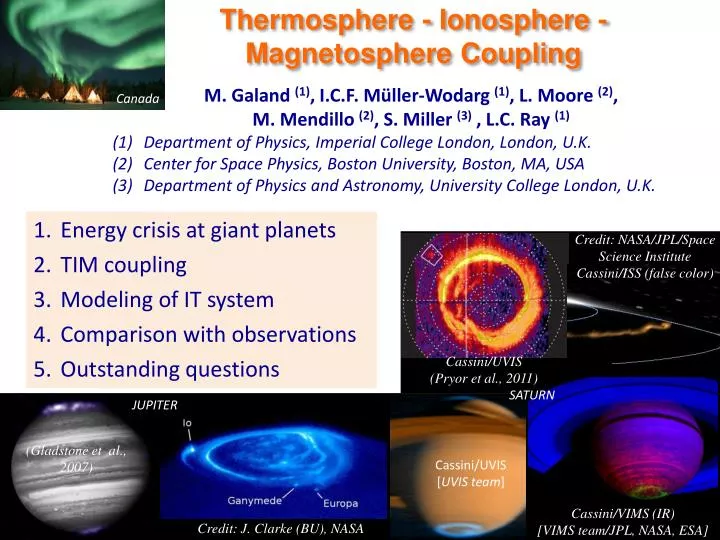
Thermosphere - Ionosphere - Magnetosphere Coupling. M. Galand (1) , I.C.F. Müller-Wodarg (1) , L. Moore (2) , M. Mendillo (2) , S. Miller (3) , L.C. Ray ( 1 ) Department of Physics, Imperial College London, London, U.K. Center for Space Physics, Boston University, Boston, MA, USA

E N D
Thermosphere - Ionosphere - Magnetosphere Coupling M. Galand(1), I.C.F. Müller-Wodarg(1), L. Moore (2), M. Mendillo(2), S. Miller (3) , L.C. Ray (1) Department of Physics, Imperial College London, London, U.K. Center for Space Physics, Boston University, Boston, MA, USA Department of Physics and Astronomy, University College London, U.K. Canada Energy crisis at giant planets TIM coupling Modeling of IT system Comparison with observations Outstanding questions Credit: NASA/JPL/Space Science Institute Cassini/ISS (false color) Cassini/UVIS (Pryor et al., 2011) SATURN JUPITER (Gladstone et al., 2007) Cassini/UVIS [UVIS team] Cassini/VIMS (IR) [VIMS team/JPL, NASA, ESA] Credit: J. Clarke (BU), NASA
SETTING THE SCENE: THE ENERGY CRISIS AT THE GIANT PLANETS
THERMAL PROFILE (EARTH) Exosphere Texo 500 km Key transition region between the space environment and the lower atmosphere Thermosphere Ionosphere 85 km Mesosphere 50 km Stratosphere ~ 15 km Troposphere
SOLAR ENERGY DEPOSITION IN THE UPPER ATMOSPHERE Solar photons ion, e- Neutral Suprathermal electrons B Thermosphere ion, e- Ionospheric e- heating Thermal e- Ne, Nion SP, SH Te * Airglow + Neutral atmospheric heating Exothermic reactions
IS THE SUN THE MAIN ENERGY SOURCE OF PLANERATY THERMOSPHERES? W Main energy source: UV solar radiation Main energy source? Outer planets Earth Exospheric temperature (K) CO2 atmospheres [after Mendillo et al., 2002]
ENERGY CRISIS AT THE GIANT PLANETS Observed values at low to mid-latitudes solstice equinox Modeled values (Sun only) [After Yelle and Miller, 2004; Melin et al., 2011 (+poster)]
ENERGY BUDGET OF THE THERMOSPHERE • HEATING SOURCES • Solar heating through excitation/dissociation/ionization + exothermic chemical reactions • Auroral particle heating via collisions + chemistry • [Grodent et al., 2001] • “Ionospheric Joule heating” via auroral electrical currents and ion-drag heating [Vasyliũnas and Song, 2005] • Dissipation of upward, propagating waves(such as gravity waves, …) • Solar EUV/FUV heating*: 0.5 TW (Earth), 0.8 TW (Jupiter), 0.2 TW (Saturn) • Auroral part./Joule heating*: 0.08 TW (Earth), 100 TW (Jupiter), 5-10 TW (Saturn) [*: Strobel, 2002]
MAGNETOSPHERE-IONOSPHERE-THERMOSPHERE COUPLING AURORAL THERMOSPHERE IONOSPHERE Exchange of particles, momen- tum & energy • Examples of ITM coupling: • Angular momentum transfer • Ion outflow, particle precipitation MAGNETOSPHERE
MAGNETOSPHERE-IONOSPHERE-THERMOSPHERE COUPLING • Overall, at high latitudes: the magnetosphere extracts angular momentum from the upper atmosphere through the magnetic field-aligned currents [e.g., Hill, 1979] • The magnetosphere “swims” on the ionosphere. MAGNETOSPHERE IONOSPHERE
MAGNETOSPHERE-IONOSPHERE-THERMOSPHERE COUPLING AURORAL THERMOSPHERE IONOSPHERE Exchange of particles, momen- tum & energy • Examples of ITM coupling: • Angular momentum transfer • Ion outflow, particle precipitation MAGNETOSPHERE
TIM coupling through current system TO MAGNETOSPHERE FROM MAGNETOSPHERE Field-aligned current S AURORAL THERMOSPHERE Field-aligned current IONOSPHERE Pedersen current QJ = J. Ei • Ionospheric Joule heating • (resistive + frictional heating) • [Vasyliũnas and Song, 2005]
MAGNETOSPHERE-IONOSPHERE-THERMOSPHERE COUPLING ATMOS Energy redistribution towards lower latitudes? MAGNETOSPHERE
Ion drag fridge mechanism [Smith et al., 2007; Smith and Aylward, 2009] EXOSPHERIC TEMPERATURE STIM Stronger heating wind direction Stronger cooling Local time averaged [Mueller-Wodarg et al., 2011] Polar sub-corotation due to auroral forcing (westward ion velocities due to ambient E fields) drives equator-to-pole circulation
Does the ion drag fridge mechanism rule out auroral energy in solving the global energy crisis at Giant Planets?
COUPLED FLUID/KINETIC STIM MODEL Solar Flux * Full ion-neutral dynamical coupling Neutral temperatures 1D Energy Deposition Model [Galand et al., JGR, 2009, 2011] 3D Thermosphere-Ionosphere Model Thermospheric densities (Nn), winds, & temp. [Müller-Wodarg et al., Icarus, 2006] Beer-Lambert Law applied to the solar flux Nn * Pe, Pi Ionospheric densities (Ne, Ni) , drifts, & temperatures (Te, Ti) [Moore et al., JGR, 2008] Boltzmann Equation applied tosuprathermal electrons Pe, Pi, Qe Ne, Te Incident Auroral Electron Distribution Electron and ion densities & temperatures Electrical conductances Electric field Flexible model which allows us to explore the parameter space and assess the effect of it on ionospheric/thermospheric quantities, such as Ne, S, Tn.
STIM RESULT 1: Ionosphericconductances in auroral regions Q0 = 0.2 mW m-2 12 LT Pedersen conductance (mho) SOLAR VALUES with Dt = 25 min • Pedersen conductivities peak at the homopauseconductances peak near 2.5 keV • - At low energies, conductances are driven by the solar source [Galand et al., 2011]
STIM RESULT 1: Ionosphericconductances in auroral regions Q0 = 0.2 mW m-2 12 LT Pedersen conductance (mho) with Dt = 25 min • Pedersen conductivities peak at the homopauseconductances peak near 2.5 keV • - At low energies, conductances are driven by the solar source [Galand et al., 2011]
STIM RESULT 1: IonosphericConductances in auroral regions Composition Altitude range SP=max(SP)/10 over 70 km (E) and 500 km (S) Strength of B field B field 20 times stronger at J cp w/ S Slippage parameter(1) for Jupiter(2) & Saturn(3): (1) Bunce et al. [2003]; (2) Cowley et al. [2004]; (3) Galand et al. [2011]
STIM RESULT 2: sensitivity to vibrationally excited H2 rate • Charge exchange reaction H+ + H2(v≥4) H2+ + H (1) controls the abundance of H3+ as it is quickly followed by: H2+ + H2 H3+ + H • Reaction rate k1* = k1 [H2(v≥4)]/[H2] • Low k1* means less charge exchange reaction and increase in ionospheric densities • k1 = 10-9 cm3 s-1 [Huestis, 2008] • At low- and mid-latitudes: Moore et al. (2010) found best match between model and Cassini RSS data for a reduction of ([H2(v≥4)]/[H2]) from Moses and Bass [2000] • In the auroral regions, expected to be larger: Galand et al. (2011) assumed 2 x ([H2(v≥4)]/[H2])from Moses and Bass [2000] • How does this affect thermospheric circulation?
STIM RESULT 2: sensitivity to vibrationally excited H2 rate EXOSPHERIC TEMPERATURE wind direction 3 cells Local time averaged [Mueller-Wodarg et al., 2011]
Implication for exospheric temperatures (1) STIM, 3 cells (2) STIM, 1 cell (3) Voyager UVS (Vervack and Moses, 2011) (4) Voyager UVS (Smith et al., 1983) (5) Cassini UVIS (Nagy et al., 2009) (6) UKIRT (Melin et al., 2007) 3 1 4 2 5 6 + [Mueller-Wodarg et al., 2011]
Sample of relevant observations: Earth-based + space missions Which observations can help constrained the problem? [e.g., Melin, talk] • Combine as many as possible to better constrain the problem
JUNO over the polar regions Credit: Juno Team Credit: Juno Team • JUNO observations through the magnetic field lines connected to the auroral ionosphere, close/within the acceleration region (expected to be 2-3 RJ from center [Ray et al., 2009]): • - Electric currents along magnetic field lines • - Plasma/radio waves revealing processing responsible for particle acceleration [see Hess, tutorial] • - Energetic particles precipitating into atmosphere creating aurora • Ultraviolet/IR auroral emissions regarding the morphology of the aurora
Outstanding questions • Can the energy crisis be solved via auroral forcing alone as proposed here? • Is the mechanism proposed efficient at Jupiter, Uranus (seasonal asymmetry [Melin et al., 2011 + poster]), and Neptune? • At Saturn, beside the solar contribution which is dominant [Moore et al., 2010], are they additional energy sources at low- and mid-latitudes? [e.g., break-down in co-rotation of the ions in the ionosphere [Stallard et al., 2010; Tao, poster; Ray, talk], molecular neutral torus of Saturn through charge-exchange (ENA) [e.g., Jurak& Johnson, 2001], wave heating (super-rotat≠IR)] Further constraints on ionospheric densities at different LT [dawn/dusk RSS, Max Ne SEDs, ground-based IR in H3+ (noon!)] • What drive the hemispheric differences observed at Saturn in the magnetosphere and auroral, ionospheric regions? • Asymmetry in B field? Hemispheric (seasonal) differences in the atmosphere? If the latter, should reverse now as going out of equinox? • Is the variable rotation rate observed in the magnetosphere linked to atmospheric dynamics? [e.g., Jia/Kivelson talk] (two-way MI coupling)
Mendillo et al. (2002) PLANETARY IONOSPHERES in the SOLAR SYSTEM Ionospheres in the solar system
ORIGIN of the soft X-RAY and UV SOLAR SPECTRUM [LASP, TIMED/SEE] Ionization Heating of thermosphere
Pedersen (sP) & Hall (sH) conductivities: with Pedersen (SP) & Hall (SH) conductances:
IONOSPHERIC CONDUCTIVITIES IN THE AURORAL REGION 12 LT Sun only (0.1 mW m-2 including 4x10⁻³mW m-2 for photoe-) Sun + Soft e- (500 eV, 0.2 mW m-2) Sun + Hard e- (10 keV, 0.2 mW m-2)
IONOSPHERIC CONDUCTANCES IN THE AURORAL REGION Em = 10 keV <Q0> = 0.2 mW m-2 0800 UT • LT-dependence based on HST/UV brightness analysis • [Lamy et al., 2009] 0400 – 1400 UT Pedersen DtP = 23 min Electrical conductances proportional to but shifted in time [Galand et al., 2011]
ENERGY REDISTRIBUTION FROM HIGH TO LOWER LATITUDES The “Ion Drag Fridge” Subcorotating Region Smith et al., Nature (2007) Smith and Aylward (2009) Pole-to-equator flow Equator-to-pole flow • Polar sub-corotation due to auroral forcing (westward ion velocities due to ambient E fields) drives equator-to-pole circulation • NOTE: this is not simply the return-flow of thermally driven pole-to-equator winds higher up! • Therefore, the poleward flow cools the equatorial regions • Does this rule out magnetospheric energy in solving the Gas Giant energy crisis?