Download
1 / 96
1k likes | 1.14k Views
This article delves into self-adjusting data structures, specifically focusing on AVL trees and their efficiency in data access. Using a given AVL tree with nodes 44, 17, 78, 32, 50, 88, 48, and 62, we analyze the performance when searching the sequence 48, 50 multiple times. We evaluate the worst-case operation time, discuss methods like Move-to-Front, Transposition, and Frequency Counter, and assess their implications for data access efficiency. Furthermore, we introduce Splay Trees and their adaptive advantages over traditional structures.

E N D
Self-adjusting Structures Consider the following AVL Tree 44 17 78 32 50 88 48 62
Self-adjusting Structures Consider the following AVL Tree 44 17 78 32 50 88 48 62 Suppose we want to search for the following sequence of elements: 48, 48, 48, 48, 50, 50, 50, 50, 50.
Self-adjusting Structures Consider the following AVL Tree In this case, is this a good structure? 44 17 78 32 50 88 48 62 Suppose we want to search for the following sequence of elements: 48, 48, 48, 48, 50, 50, 50, 50, 50.
Self-adjusting Structures • So far we have seen: • BST: binary search trees • Worst-case running time per operation = O(N) • Worst case average running time = O(N) • Think about inserting a sorted item list • AVL tree: • Worst-case running time per operation = O(logN) • Worst case average running time = O(logN) • Does notadapttoskewdistributions
Self-adjusting Structures • The structure is updated after each operation • Consider a binary search tree. If a sequence of insertions produces a leaf in the level O(n), a sequence of m searches to this element will represent a time complexity of O(mn) Use an auto-adjusting strucuture
Self adjustablelists • Move to Front • Whenever an element is accessed it is moved to the front of the list • Transposition • Whenever an element x is accessed, we switch x with its predecessor • Frequency counter • The list is always sorted by decreasing order of frequencies
Self adjustablelists EXAMPLE
Self-adjusting Structures • AlgoritmosAdmissíveis • Um método é dito admissível se no i-ésimo acesso ele move o elemento acessado ki posições para frente • Classe de algoritmos que engloba todos os métodos apresentados.
Análise do Move to Front Teorema. Seja H um método admissível e seja s uma sequência de m acessos. Então CustoMF(S) <= 2CustoH(s) –m, Aonde CustoMF(S) e CustoH(s) são, respectivamente, os custos de MF e H para processar uma sequência s de requisições
Análise do Move to Front Prova. Empregamos o método da função potencial Di :o numero de inversões da lista mantida pelo MF em relação a lista do algoritmo H após o i-ésimo acesso. Lista de H: a b c f e d Lista de MF: b a f d e c Inversões: (b,a) , (f,c), (d,e), (d,c) Di =4 Temos que c’i= ci+Di–Di-1
Análise do Move to Front Prova. Elemento x é acessado pelo MF. x: k-ésimo elemento da lista de H x: j-ésimo elemento da lista de MF p: número de elementos que precedem x na lista de MF e sucedem x na lista de H • Quando o MF coloca x na primeira posição, j-1-p inversões são criadas e p são destruídas • Quando H move o elemento x ei operações para frente, ei inversões são destruídas e nenhuma é criada
Análise do Move to Front Prova. Da análise anterior c’i = j +(j-1-p) – (p + ei) = 2(j-1-p) - ei + 1 Temos que j-1-p <=k-1 já que o número de inversões criadas é limitado pela posição de x na lista de H. Logo, c’i <= 2(k-1) - ei + 1 Somando c’i Segue que
BadSequences for TranspositionandFrequencyCounter • Transposition • We insert n elements a1,…,an and then we access the element an n times. • Transposition pays O(n2) while MF pays O(n) • Frequency Counter • List with elements (an,…,a1). We access an n times, an-1 (n-1) times and so on. FC does not reorganize the list. • FC pays O(n3) while MF pays O(n2)
Further Reading Randomization avoids malicious adversaries
Self-adjusting Structures SplayTrees (TarjanandSleator 1985) • Binarysearch tree. • Everyaccessed node isbroughttothe root • Adapttotheaccessprobability distribution
Splay trees: Basic Idea • Try to make the worst-case situation occur less frequently. • In a Binary search tree, the worst case situation can occur with every operation. (while inserting a sorted item list). • In a splay tree, when a worst-case situation occurs for an operation: • The tree is re-structured (during or after the operation), so that the subsequent operations do not cause the worst-case situation to occur again.
Splay trees: Basic idea • The basic idea of splay tree is: • After a node is accessed, it is pushed to the root by a series of AVL tree-like operations (rotations). • For most applications, when a node is accessed, it is likely that it will be accessed again in the near future (principleoflocality).
Afirstattempt • A simple idea • When a node k is accessed, push it towards the root by the following algorithm: • On the path from k to root: • Do a singe rotation between node k’s parent and node k itself.
Afirst attempt k5 Accessing node k1 k4 F k3 E k2 D k1 A B B access path
Afirst attempt k5 After rotation between k2 and k1 k4 F k3 E k1 D k2 C A B
Afirst attempt After rotation between k3 and k1 k5 k4 F k1 E k3 k2 A B C D
Afirst attempt After rotation between k4 and k1 k5 k1 F k4 k2 k3 E A B C D
Afirstattempt k1 k1 is now root k5 k2 k4 A B F E k3 C D But k3 is nearly as deep as k1 was. An access to k3 will push some other node nearly as deep as k3 is. So, this method does not work ...
Splaying - algorithm • Assume we access a node. • We will splay along the path from access node to the root. • At every splay step: • We will selectively rotate the tree. • Selective operation will depend on the structure of the tree around the node in which rotation will be performed
Implementing Splay(x, S) • Do the following operations until x is root. • ZIG: If x has a parent but no grandparent, then rotate(x). • ZIG-ZIG: If x has a parent y and a grandparent, and if both x and y are either both left children or both right children. • ZIG-ZAG: If x has a parent y and a grandparent, and if one of x, y is a left child and the other is a right child.
Implementing Splay(x, S) • Do the following operations until x is root. • ZIG: If x has a parent but no grandparent, then rotate(x). • ZIG-ZIG: If x has a parent y and a grandparent, and if both x and y are either both left children or both right children. • ZIG-ZAG: If x has a parent y and a grandparent, and if one of x, y is a left child and the other is a right child. y x C A B
Implementing Splay(x, S) • Do the following operations until x is root. • ZIG: If x has a parent but no grandparent, then rotate(x). • ZIG-ZIG: If x has a parent y and a grandparent, and if both x and y are either both left children or both right children. • ZIG-ZAG: If x has a parent y and a grandparent, and if one of x, y is a left child and the other is a right child. root x y y A x C ZIG(x) A B B C
Implementing Splay(x, S) • Do the following operations until x is root. • ZIG: If x has a parent but no grandparent, then rotate(x). • ZIG-ZIG: If x has a parent y and a grandparent, and if both x and y are either both left children or both right children. • ZIG-ZAG: If x has a parent y and a grandparent, and if one of x, y is a left child and the other is a right child. root y x x A y C ZAG(x) A B B C
Implementing Splay(x, S) • Do the following operations until x is root. • ZIG: If x has a parent but no grandparent, then rotate(x). • ZIG-ZIG: If x has a parent y and a grandparent, and if both x and y are either both left children or both right children. • ZIG-ZAG: If x has a parent y and a grandparent, and if one of x, y is a left child and the other is a right child. z y D x C A B
x y A z B D C Implementing Splay(x, S) • Do the following operations until x is root. • ZIG: If x has a parent but no grandparent, then rotate(x). • ZIG-ZIG: If x has a parent y and a grandparent, and if both x and y are either both left children or both right children. • ZIG-ZAG: If x has a parent y and a grandparent, and if one of x, y is a left child and the other is a right child. z y D ZIG-ZIG x C A B
Implementing Splay(x, S) • Do the following operations until x is root. • ZIG: If x has a parent but no grandparent, then rotate(x). • ZIG-ZIG: If x has a parent y and a grandparent, and if both x and y are either both left children or both right children. • ZIG-ZAG: If x has a parent y and a grandparent, and if one of x, y is a left child and the other is a right child. z y A x D B C
z x y z y A x D A B C D B C Implementing Splay(x, S) • Do the following operations until x is root. • ZIG: If x has a parent but no grandparent, then rotate(x). • ZIG-ZIG: If x has a parent y and a grandparent, and if both x and y are either both left children or both right children. • ZIG-ZAG: If x has a parent y and a grandparent, and if one of x, y is a left child and the other is a right child. ZIG-ZAG
Splay Example Apply Splay(1, S) to tree S: 10 9 8 7 6 ZIG-ZIG 5 4 3 2 1
1 2 3 Splay Example Apply Splay(1, S) to tree S: 10 9 8 7 6 ZIG-ZIG 5 4
1 4 5 2 3 Splay Example Apply Splay(1, S) to tree S: 10 9 8 7 6 ZIG-ZIG
Splay Example Apply Splay(1, S) to tree S: 10 9 8 1 ZIG-ZIG 6 7 4 2 5 3
1 8 6 9 7 4 2 5 3 Splay Example Apply Splay(1, S) to tree S: 10 ZIG
1 10 8 6 9 7 4 2 5 3 Splay Example Apply Splay(1, S) to tree S:
Apply Splay(2, S) to tree S: 2 1 10 1 8 4 8 10 3 6 6 9 9 Splay(2) 7 4 5 7 2 5 3
Splay Tree Analysis • Define thepotentialfunction • Associate a positive weighttoeach node v: w(v) • W(v)= w(y), y belongsto a subtreerootedat v • Rank(v) = log W(v)
Splay Tree Analysis • Define thepotentialfunction • Associate a positive weighttoeach node v: w(v) • W(v)= w(y), y belongsto a subtreerootedat v • Rank(v) = log W(v) • The treepotentialis: rank(v) v
Upperbound for theamortized time ofa complete splayoperation • Toestimatethe time of a splayoperationwe are goingto use thenumberofrotations
Upperbound for theamortized time ofa complete splayoperation • Toestimatethe time of a splayoperationwe use thenumberofrotations Lemma: The amortized time for a complete splayoperationof a node x in a treeof root r isatmost 1 + 3[rank(r) – rank(x)] whererank(x) istherankof x beforethesplayand rank(r) istherankof r afterthesplay.
Upperbound for theamortized time ofa complete splayoperation Proof: The amortized cost a is given by a=t + after– before t : number of rotations executed in the splaying
Upperbound for theamortized time ofa complete splayoperation Proof: The amortized cost a is given by a=t + after– before a = o1 + o2 + o3 + ... + ok oi : amortized cost of the i-th operation during the splay ( zig or zig-zig or zig-zag)
Upperbound for theamortized time ofa complete splayoperation Proof: i : potentialfunctionafter i-thoperation ranki:rankafter i-thoperation oi = ti+ i –i-1
Splay Tree Analysis • Operations • Case 1: zig( zag) • Case 2: zig-zig (zag-zag) • Case 3: zig-zag (zag-zig)
Splay Tree Analysis • Case 1: Only one rotation (zig) root r x
Splay Tree Analysis • Case 1: Only one rotation (zig) root r x w.l.o.g. x r r A x C ZIG(x) A B B C