Earth Sciences Division – Hydrosphere, Biosphere, and Geophysics

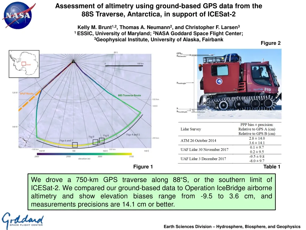
1. Assessment of altimetry using ground-based GPS data from the88S Traverse, Antarctica, in support of ICESat-2 Kelly M. Brunt1,2, Thomas A. Neumann2, and Christopher F. Larsen3 1 ESSIC, University of Maryland; 2NASA Goddard Space Flight Center;3Geophysical Institute, University of Alaska, Fairbank Figure 2 Figure 1 Table 1 We drove a 750-km GPS traverse along 88∘S, or the southern limit of ICESat-2. We compared our ground-based data to Operation IceBridge airborne altimetry and show elevation biases range from -9.5 to 3.6 cm, and measurements precisions are 14.1 cm or better. Earth Sciences Division – Hydrosphere, Biosphere, and Geophysics

2. Name: Kelly Brunt, Cryospheric Sciences Lab, NASA GSFC and ESSIC, University of Maryland E-mail: kelly.m.brunt@nasa.gov Phone: 301-286-5943 References: Brunt, K.M., Neumann, T.A., & Larsen, C.F. (accepted). Assessment of altimetry using ground-based GPS data from the 88S Traverse, Antarctica, in support of ICESat-2. The Cryosphere. doi.org/10.5194/tc-13-1-2019 Data Sources: NASA Operation IceBridge ATM (2014, 2016); NASA Operation IceBridge UAF Lidar (2017); Digital Globe WorldView-2 imagery Technical Description of Figures: Figure 1: Map of the 750-km 88S Traverse Route; color indicates elevation. The segment along 88S (intersecting ICESat-2 ground tracks) is ~300 km. The South Pole Operational Traverse (SPoT) Route is also indicated in orange. Figure 2: One of the traverse vehicles and the GPS configuration on that vehicle. Table 1: Summary of measurement results for the 2 lidars assessed in this analysis. Elevation accuracies and surface measurement precisions are reported as a residual, following the convention of mean bias ± 1σ standard deviation, or 0.0 ± 0.0 cm. Scientific significance, societal relevance, and relationships to future missions: We collected a long length-scale of GPS elevation data for ground-based validation of satellite elevation data. Further, our traverse route intersects 20% of the ICESat-2 reference ground tracks that span the 91-day repeat cycle; comparing different orbits separated by many days gives us a chance to assess uncorrelated error in ICESat-2. Ultimately, this article presents a highly accurate ground-based dataset for evaluation of ICESat-2 surface elevations. It also provides an assessment of OIB altimeters that will in turn be used to provide assessments of ICESat-2 accuracy. Earth Sciences Division – Hydrosphere, Biosphere, and Geophysics

3. Comparison of multi-angle polarimeters in the PODEX field campaignKirk Knobelspiesse1, Qian Tan2, Carol Bruegge3, Brian Cairns4, Jacek Chowdhary4, Bastiaan van Diedenhoven4, David Diner3, Richard Ferrare5, Gerard van Harten3, Veljko Jovanovic3, Matteo Ottaviani4, Jens Redemann6, Felix Seidel3 and Kenneth Sinclair4 1GSFC, code 616 2NASA ARC, 3JPL, 4GSFC, code 611 5NASA LaRC6Univ. Oklahoma Bland-Altman Limits of Agreement: For each comparison pair, normalize by the paired measurement uncertainty, then plot against the mean paired value. Calculate the mean and standard deviation, which are used to find the Limits of Agreement, within which 95% of the data reside. If these values are greater than +/- 1.96 in normalized uncertainty space, then measurements do not agree within the expected uncertainty. The POlarimeterDEfinitionEXperiment (PODEX) deployed multiple polarimeters and lidars in early 2013 on the ER-2 aircraft, based NASA AFRC. Polarimeters have widely varying designs, capabilities and measurement accuracies, which must be validated and compared. Despite their common usage, metrics such as correlation coefficients and root-mean square error are not appropriate for assessment of the question: Do observations agree within stated uncertainties? We used the Bland-Altman Limits of Agreement, which is statistically robust and appropriate for datasets with varying measurement uncertainty. We found that, while polarimeters do agree within uncertainty expectations in most cases, there is possibly a calibration error in one band, and uncertainty expectations may need to be increased for some scene types. Research Scanning Polarimeter RSP (GISS), prototype for Glory/APS Airborne Multiangle SpectroPolarimetric Imager AirMSPI (JPL), prototype for MAIA Polarimeters Earth Sciences Division – Hydrosphere, Biosphere, and Geophysics

4. Name: Kirk Knobelspiesse, Code 616, Ocean Ecology Laboratory, NASA GSFC E-mail: kirk.d.knobelspiesse@nasa.gov Phone: 301-614-6242 References: Knobelspiesse, K., Q. Tan, C. Bruegge, B. Cairns, J. Chowdhary, B. van Diedenhoven, D. Diner, R. Ferrare, G. van Harten, V. Jovanovic, M. Ottaviani, J. Redemann, F. Seidel, and K. Sinclair. 2019. "Intercomparison of airborne multi-angle polarimeter observations from the Polarimeter Definition Experiment." Applied Optics, 58 (3): 650 [10.1364/ao.58.000650] Data Sources: The first author was supported in this research by the ACE Mission Study. The research was conducted at both the NASA Ames Research Center in Moffett Field, California, and the NASA Goddard Space Flight Center in Greenbelt, Maryland. Technical Description of Figure: Uncertainty normalized RSP–AirMSPI difference (D), plotted with respect to (xRSP + xAirMSPI) / 2, for reflectance (left) and the Degree of Linear Polarization (DoLP) (right). Normalization is performed to account for variable measurement uncertainty. Color denotes the comparison channel, such that 470 nm is blue, 660/670 nm is green, and 865 nm is red. Symbols indicate the comparison scene (see Knobelspiesse et al, 2019), while horizontal and dashed solid lines indicate D = 0 and D +/- 1.96, respectively. Roughly 95% of comparisons should fall within the dashed lines. DoLP shows a significant positive correlation, so limits of agreement (LOA) were not calculated until the data were further split into different scene types. This figure better visualizes the relationship between observations than a standard scatterplot, and incorporates variable measurement uncertainty. Scientific significance, societal relevance, and relationships to future missions: While we find that these polarimeters largely agree as expected, we demonstrate simple statistical comparison metrics that are more appropriate than the correlation or root mean square error metrics frequently, but incorrectly, applied. Earth Sciences Division – Hydrosphere, Biosphere, and Geophysics

5. Lake Chad: dry season area projections through the year 2100 Fritz Policelli1, Ben Zaitchik2, Hahn Jung1, Alfred Hubbard3, Charles Ichoku4 1Code 617 NASA GSFC, 2Johns Hopkins University, 3Code 618 NASA GSFC, 4Howard University Projections of Lake Chad dry season area through 2100. Based on CMIP5 model precipitation and evapotranspiration and regression based model of area. Left RCP 2.6, Right RCP 8.5. Contrary to speculation, the lake does not disappear (at least not during the dry season). Earth Sciences Division – Hydrosphere, Biosphere, and Geophysics

6. Name: Fritz Policelli, Code 617, NASA GSFC E-mail: fritz.s.policelli@nasa.gov Phone: 301-614-6573 • References: • Policelli, F, Zaitchik, B., Hubbard, A., Jung, H., Ichoku, C., 2019 submitted, Projections of Lake Chad total surface water area derived by forcing a statistical model of the lake area with results of climate simulations through the year 2100, Climatic Change • Leblanc, M., Lemoalle, J., Bader, J.-C., Tweed, S., Mofor, L., 2011. Thermal remote sensing of water under flooded vegetation: New observations of inundation patterns for the ‘Small’ Lake Chad. Journal of Hydrology 404, 87–98. https://doi.org/10.1016/j.jhydrol.2011.04.023 • Magrin, G. The disappearance of Lake Chad: history of a myth. J Political Ecology 2016, 23, 204–222. • Data Sources: Terra MODIS, FEWSNET (ET), CHIRPS (precip), CMIP5 Models (KNMI Climate Explorer), ESA Sentinel 1 C-band radar, Lake Chad area estimates from Leblanc et al., 2011 • Technical Description of Figures: • Graphics: CMIP5 climate model based projections of Lake Chad dry season area through 2100. The average is in black. • Graphic 1: Results from 74CMIP5 RCP2.6 climate models. Note the slight downward trend of area. • Graphic 2: Results from 85CMIP5 RCP8.5 climate models. Note the slight upward trend of area. • Scientific significance, societal relevance, and relationships to future missions: The paper provides projections of Lake Chad dry season area which could help inform discussions in the popular media and at international conferences about engineering an inter-basin transfer of water from the Congo River Basin to Lake Chad because of concern that the lake will dry up (Magrin, 2016). Future missions and modeling efforts could improve the uncertainty of these projections. Earth Sciences Division – Hydrosphere, Biosphere, and Geophysics

7. Forest Regrowth as a Driver of the Global Terrestrial Carbon Sink B. Poulter, Biospheric Sciences, T. Pugh, Univ Birmingham, M. Lindeskog, Lund Univ., B. Smith, W Sydney Univ., A. Alneth, Karlsruhe Inst. Tech., V. Haverd, CSIRO, & L.Calle, Montana State Univ. Regrowth area (fraction) Figure 1 Figure 2 Forest demography determines forest structure, which is a key driver in explaining how forests mitigate increases in atmospheric carbon dioxide. • Earth Sciences Division – Hydrosphere, Biosphere, and Geophysics

8. Name: B. Poulter, Biospheric Sciences, NASA GSFC E-mail: benjamin.poulter@nasa.gov Phone: 301-614-6659 References: Pugh, T, M Lindeskog, B Smith, B Poulter, A Arneth, V Haverd, and L Calle. 2019. The role of forest regrowth in global carbon sink dynamics. Proceedings of the National Academy of Science, DOI:10.1073/pnas.1810512116. Poulter, B, L Aragão, N Andela, V Bellassen, P Ciais, T Kato, X Lin, B Nachin, S Luyssaert, N Pederson, P Peylin, S Piao, T Pugh, S Saatchi, D Schepaschenko, M Schelhaas, A Shivdenko. 2019. The global forest age dataset and its uncertainties (GFADv1.1). NASA National Aeronautics and Space Administration, PANGAEA, https://doi.org/10.1594/PANGAEA.897392 Le Quéré, C, RM Andrew, P Friedlingstein, S Sitch, J Pongratz, AC Manning, JI Korsbakken, GP Peters, JG Canadell, RB Jackson, TA Boden, PP Tans, OD Andrews, VK Arora, DCE Bakker, L Barbero, M Becker, RA Betts, L Bopp, F Chevallier, LP Chini, P Ciais, CE Cosca, J Cross, K Currie, T Gasser, I Harris, J Hauck, V Haverd, RA Houghton, CW Hunt, G Hurtt, T Ilyina, AK Jain, E Kato, M Kautz, RF Keeling, K Klein Goldewijk, A Körtzinger, P Landschützer, N Lefèvre, A Lenton, S Lienert, I Lima, D Lombardozzi, N Metzl, F Millero, PMS Monteiro, DR Munro, JEMS Nabel, S I Nakaoka, Y Nojiri, XA Padin, A Peregon, B Pfeil, D Pierrot, B Poulter, et al. 2018. Global Carbon Budget 2017. Earth System Science Data, 10:405-448. Kondo, M., K Ichii, PK Prabir, B Poulter, L Calle, C Koven, TAM Pugh, E Kato, A Harper, S Zaehle, and A Wiltshire. 2018. Plant regrowth as a driver of recent enhancement of terrestrial CO2 uptake. Geophysical Research Letters, 45(10):4820-4830. Data Sources: National forest inventory data; ICESAT-1 GLAS lidar returns; MODIS c5.1 Land Cover; Climate Research Unit met. data; Technical Description of Images: Figure 1. Fraction of forest defined as regrowth (less than 140-y-old) in the global forest age dataset, GFADv1.1, for year 2010. Figure 2. Total net ecosystem production (NEP) for primary / intact forest and regrowth forest. Regrowth forest NEP is partitioned to demographic (dark green) and climate+CO2 (light green). Symbols represent uncertainty in the NEP flux from forest management assumptions. Scientific significance: This is the first study to attribute the role of forest demography on the terrestrial carbon sink using process-based dynamic global vegetation models and a new global forest age database. Previous work has alluded to demography being an important driver and here we directly test this hypothesis using novel model and data methods. Relevance for future science and relationship to Decadal Survey: We plan to update the global forest age dataset (GFADv1.1) using ICESAT-2 and GEDI forest structure measurements in FY19, and using techniques developed with Worldview stereo-imagery to estimate tree height and age relationships. The work directly addresses the Decadal Survey by providing insights into the drivers responsible for terrestrial carbon storage and fluxes, and will be further developed from data expected to be provided by Designated Observables Surface Biology and Geology, and Surface Deformation and Change. Earth Sciences Division – Hydrosphere, Biosphere, and Geophysics

9. Recovered Apollo 15 & 17 Heat Flow Data and their Interpretation Patrick T. Taylor1 1Geodesy and Geophysics Lab, NASA GSFC Figure 1 Figure 2 Apollo missions 15 (Figure 1) and 17 (Figure 2) deployed thermal sensors in the regolith to measure the lunar heat flow. Figure 1 & 2 show the temperature vs. time for Apollo15 and 17, respectively. Data from 1971 through 1974 were processed by the PI, Mark Langseth. Data from 1975 -1977 were only recently recovered under LASER and P-DART grants. These recovered data confirmed the result that the heat flow was increasing with time, an anomalous result. However, using these recovered data we determined that the increase in temperature was due to a change in the albedo by the astronaut footprints. Earth Sciences Division – Hydrosphere, Biosphere, and Geophysics

10. Name: Patrick T. Taylor, Geodesy and Geophysics Lab, NASA GSFC E-mail: Patrick.t.taylor@nasa.gov Phone: 301-614-6454 References: S. Nagihara, W.S. Kiefer, P.T. Taylor, D.R. Williams and Y. Nakamura, 2018: Examination of the Long-Term Subsurface Warming Observed at the Apollo 15 and 17 Sites Utilizing the Newly Restored Heat Flow Experiment Data From 1975 to 1977. JGR (Solid Earth), doi.org/10.1029/2018JE005579 M.G. Langseth, 1977: Lunar heat-flow experiment: Final technical report (p.289). Palisades, New York Lamont-Doherty Geological Observatory. Data Sources: These data were recovered from various sources mainly the Washington and Fort Worth National Record Centers, JSC and LPI. Technical Description of Figures: Figure 1: Temperature vs time record for the Apollo 15 heat flow probe. The data from July 1972 through 1974 were interpreted and published by the PI Mark Langseth and his collaborators. The data from December 1975 through 1977 were restored and presented in the JGR paper and sent to the NSSDCA. Figure 2: Temperature versus time record for the Apollo 17 heat flow probe. This probably started recording December 1972 through 1977 when the instruments were turned off. The data from 1975 through 1977 were recovered and interpreted in our paper. Scientific significance, societal relevance, and relationships to future missions: By recovering the Apollo mission heat flow data they were not only found to be valuable lunar data but we were able to solve the long standing problem of why the temperature versus depth values were increasing over time. Future lunar and planetary missions will have to solve the problem of assuring that the emplacement of the probes do not disturb the surrounding regolith. Our paper was called out in two Research Highlights, one in Nature, “Lunar crews left thermal print.” and one in EOS, “The Case of the Missing Lunar Heat Flow Data is Finally Solved.” Earth Sciences Division – Hydrosphere, Biosphere, and Geophysics